Материал: [2.1] 3D Imaging, Analysis and Applications-Springer-Verlag London (2012)
6 3D Shape Registration |
225 |
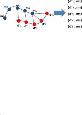
Fig. 6.3 Correspondence estimation in ICP. For each transformed data point
di = Rdi + t the closest model point mj is estimated (left). The list of corresponding points is then defined (right)
More specifically, the value
i |
= |
i + |
t) |
− |
m |
j |
|
e2 |
(Rd |
|
|
2 |
(6.4) |
is the square of the residual. Figure 6.3 illustrates the step of correspondence computation. For each data point (in red) the closest model point (in blue) is computed using the Euclidean distance. The list of correspondences is thus obtained. Note that, given point correspondences, the computation of R and t to minimize EICP in Eq. (6.2) can be solved in closed-form [78]. Several approaches are possible for the closed-form, least-squares estimation of this 3D rigid body transformation. These include approaches based on singular value decomposition (SVD), unit quaternion, dual quaternion, and orthonormal matrices. Although the study of Eggert et al. [30] found little difference in the accuracy and robustness of all these approaches, perhaps the most well-known of these is the SVD approach by Arun et al. [3]. Here, the cross-covariance matrix is formed for the Nd correspondences, (di , mj ), as
C = 1
Nd
Nd |
− ¯ |
− ¯ |
|
di |
|
||
d mj |
m T , |
(6.5) |
i=1
where the means d¯ |
¯ |
correspondences. Performing the |
, m are formed over the Nd |
||
SVD of C gives us: |
|
|
|
USVT = C |
(6.6) |
where U and V are two orthogonal matrices and S is a diagonal matrix of singular values. The rotation matrix R can be calculated from the orthogonal matrices as:
R = VUT . |
(6.7) |
Umeyama states that this solution may fail to give a correct rotation matrix and give a reflection instead when the data is severely corrupted [94]. Thus, it can be modified to always return a correct rotation matrix [94]:
|
R = VS UT , |
|
(6.8) |
|||
where |
|
|
|
|
|
|
|
|
|
if det(U) det(V) = 1 |
|
||
S = |
I |
− |
1) |
1. |
||
Diag(1, 1, . . . , 1, |
if det(U) det(V) |
= − |
||||
|
|
|
|
|
||
226 |
U. Castellani and A. Bartoli |
Once the rotation matrix has been estimated, the translation vector t can be estimated as:
t |
= ¯ |
− |
Rd¯ . |
(6.9) |
m |
|
The ICP algorithm is iterative because it iteratively improves the tentative correspondences. If true correspondences were known, clearly the process could operate in one pass. ICP has two main steps in its inner loop: (i) closest point computation and (ii) rigid transformation estimation. In more detail, the algorithm operates as follows:
1.For each data-point di D, compute the closest point mj M according to Eq. (6.3).
2.With the correspondences (di , mj ) from step 1, estimate the new transformation parameters a = (R, t).
3.Apply the new transformation parameters a from step 2 to the point cloud D.
4.If the change in EICP(a, D, M) between two successive iterations is lower than a threshold then terminate, else go to step 1.
It was proven [7] that this algorithm is guaranteed to converge monotonically to a local minimum of Eq. (6.2). Note that, as for any local iterative method, a strategy for initializing a must be used. An overview of the most popular initialization strategies is given in Sect. 6.2.3.1.
6.2.3 ICP Extensions
Although ICP has been successfully applied to many registration problems, there are several critical issues that need to be taken care of. In particular, ICP performs well when the following assumptions are met:
1.The two views must be close to each other. If not, ICP will probably get stuck in a local minimum. This issue is typically solved by pre-alignment of the two 3D views, also called coarse registration.
2.The two views must fully overlap or the data-view D must be a subset of the model-view M. The problem arises from the fact that ICP always assigns a closest model point to every data point. If a data point has no corresponding model point, this will create a spurious correspondence, an outlier with respect to the sought transformation, that will bias the solution or prevent the algorithm from finding the correct transformation parameters.
Two other important issues are the speed of computation and the accuracy of the ICP algorithm. Typically, methods focused on speed improvement try to speed up the closest point computation step, which is the bottleneck of the algorithm. Other interesting approaches address the speed of convergence by proposing new distance formulations for the problem described by Eq. (6.1). Methods focusing on accuracy exploit additional information in order to measure the similarity between corresponding points not only in terms of proximity. In the following, we describe
6 3D Shape Registration |
227 |
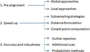
Fig. 6.4 A taxonomy of some ICP extensions
some registration techniques which improve the basic ICP method in several ways. Figure 6.4 illustrates the proposed taxonomy of ICP extensions so as to easily understand the organization of previous work in this field.
6.2.3.1 Techniques for Pre-alignment
The aim of pre-alignment techniques is to estimate a coarse transformation which will allow the two views to get closer. This helps the data-view to be transformed within the basin of attraction of the correct local minimum. In practice, instead of searching dense point-to-point correspondences, pre-alignment techniques estimate the best matching between features extracted from the views. Roughly speaking the features can be global or local. The former is a compact representation that effectively and concisely describes the entire view. The latter is a collection of local and discriminative descriptors computed on subparts of the views.
Global Approaches Typically global approaches estimate and match the principal coordinate system of each view. The simplest approach is to compute the main translational alignment by shifting the centroids of the two point clouds to the origin of the coordinate system (i.e. zero-mean). In order to estimate the orientation of the principal axes, Principal Component Analysis (PCA) can be performed on the point clouds. The problems with PCA as a pre-alignment method are (i) a 180 degree ambiguity in the direction of the principal axes, (ii) principal axes may switch for shapes that have eigenvalues similar in value, particularly if the object is able to deform slightly, (iii) a vulnerability to outliers in the raw shape data (as discussed). Even if we enforce a right handed frame using the sign of the cross-product of basis vectors, there still exists an overall 180 degree ambiguity, unless higher order moments are used. Moments of higher orders are also useful to improve accuracy [11]. Of course, these approaches perform well when the two views fully overlap. Otherwise, the non-overlapping parts change the estimation of the principal axes and thus affect the pre-alignment. Some improvements have been made by extracting and matching the skeletons of the views [20, 60] but this is feasible for articulated objects only.
228 |
U. Castellani and A. Bartoli |
Local Approaches Local approaches define a descriptor (or signature) for each 3D point which encodes local shape variation in the point neighborhood [16, 47, 49, 62, 89]. Point correspondences are then obtained as the best matches in regard of the point signatures. Various methods to compute signatures were proposed. In their seminal work [47], Johnson and Hebert introduced Spin Images. In a spin-image, the neighbors of some selected 3D point (e.g. a 3D interest point) are binned in a 2D cylindrical-polar coordinate system. This consists of a distance from the selected point within that point’s tangent plane and a signed height above/below the tangent plane. Thus the spin-image is a 2D histogram of 3D shape, where one dimension of information is sacrificed for pose invariance. In [50] curvilinear features on the object are estimated from a small amount of points of interest. Gaussian and mean curvatures are used to this aim. Similarly, in [99], bitangent curve pairs were used as landmarks on the surface. In [62] a geometric scale-space analysis of 3D models was proposed from which a scale-dependent local shape descriptor was derived. Similarly, in [16], registration involves few feature points by extending the approach for salient point detection to the 3D domain. A generative model is then estimated as a point descriptor by using Hidden Markov Models (HMMs). In [49] the proposed descriptor encodes not only local information around the point, but also inter-point relationships. The method is inspired by the so-called Shape Context [5] which was improved using the Bag-of-Words paradigm [26]. Note that from the analysis of inter-point relationships it is also possible to estimate the overlapping region between two views. It is worth noting that, in general, the estimation of the overlap area is not trivial. An interesting approach was proposed in [82] by combining local geometric features with advanced graph matching techniques. The method consists of representing all tentative point matches as a graph, and then selecting as many consistent matches among them as possible. To this aim, a global discrete optimization problem is proposed based on the so called maximum strict sub-kernel algorithm [81].
6.2.3.2 Techniques for Improving Speed
The speed of the algorithm is crucial for many applications. Unfortunately, when the number of points is very high, the basic ICP algorithm becomes very slow. In order to address this issue several strategies have been proposed, which we now outline.
Subsampling Subsampling can be applied to either the data-view only or to both the data-view and the model-view. Random and uniform strategies are common approaches [78]. Normal space sampling is a more sophisticated approach based on choosing points such that the distribution of normals among the selected points is as spread as possible. This increases the influence of smaller details which are crucial to better disambiguate the rigid transformation due to translational sliding.
Closest Point Computation As mentioned above, closest point computation is the bottleneck of the registration process due to the quadratic complexity (O(n2))
6 3D Shape Registration |
229 |
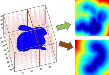
Fig. 6.5 Using the distance transform. The model-view is enclosed in a volumetric grid (left). For each point of the grid the closest model-point is computed. Two planes are highlighted on the XY and Y Z axes respectively and the distance transform values of each grid-point are visualized for both planes (right). The cyan color indicates low distance values, close to the object surface. Blue colors are negative and inside the object, darker blue meaning further from the surface. Other colors are outside the object and, as we move through the green, yellow and red colors, we move further from the surface
in finding the correspondence of each point. Early strategies were based on the organization of the model-points in a k-d tree [87] structure in order to reduce the closest point complexity to O(n log n). Closest point caching [87] also accelerates the speed of ICP (the data point correspondence search is only among a subset of model points which were the closest at the previous iteration). Indeed, in [63] k-d tree and caching are combined in order to further improve the speed of ICP. Other more effective approaches are based on the so called reverse calibration paradigm [8]. The idea is to project the source data point onto the destination model-view which is encoded as a range image [76]. In particular, the projection from the 3D domain into the range image is performed by using the calibration parameters of the 3D scanner. In this fashion the correspondence is computed in one-shot. The reverse calibration approach is especially effective for real-time application. For instance in [77] the authors proposed a real-time 3D model reconstruction system, and in [18] on-line registration is performed to build a 3D mosaic of the scene in order to improve the navigation in underwater environments. Also, one-shot computation can be carried out on a generic point cloud (not necessary coming from a range image) by precomputing the so called distance transform of the model view [32]. Figure 6.5 illustrates the distance transform. In practice, the distance to closest model-points are precomputed for all grid-points of the discretized volume. The case for using a distance transform computed for the model is particularly compelling when one wishes to align many instances of data scan to the same model scan.