Материал: [2.1] 3D Imaging, Analysis and Applications-Springer-Verlag London (2012)

the surface [21], (iii) Thin-Plate Splines (TPS) [24, 76], or (iv) linear blend skinning model (LBS) [22]. The error function can be optimized by the Levenberg-Marquardt Algorithm [51], GraphCuts [21], or Expectation-Maximization (EM) [22, 24, 61]. In [42] deformable registration is solved by alternating between correspondence and deformation optimization. Assuming approximately isometric deformations, robust correspondences are generated using a pruning mechanism based on geodesic consistency.

Deformable alignment to account for errors in the point clouds obtained by scanning a rigid object is proposed in [12, 13]. Also, in this case, the authors use TPS to represent the deformable warp between a pair of views, that they estimate through hierarchical ICP [76].

Probabilistic Methods Using probabilistic methods the uncertainty on the correct surface transformation can be addressed by adopting maximum likelihood estimation [2, 28, 41, 46, 61, 96]. Probabilistic approaches are based on modeling each of the point sets by a kernel density function [93]. The dissimilarity among such densities is computed by introducing appropriate distance functions. Registration is carried out without explicitly establishing correspondences. Indeed, the algorithm registers two meshes by optimizing a joint probabilistic model over all point-to-point correspondences between them [2]. In [46], the authors propose a correlation-based approach [93] to point set registration by representing the point sets as Gaussian Mixture Models. A closed-form solution for the L2 norm distance between two Gaussian mixtures makes fast computation possible. In [96], registration is carried out simultaneously for several 3D range datasets. The method proposes an information-theoretic approach based on the Jensen-Shannon divergence measure. In [61], deformable registration is treated as a Maximum Likelihood estimation problem by introducing the Coherent Point Drift paradigm. Smoothness constraints are introduced based on the assumption that points close to one another tend to move coherently over the velocity field. The proposed energy function is minimized with the EM algorithm. A similar approach has been proposed in [28] to track the full hand motion. A stereo set-up is employed to estimate the 3D surface. To improve the estimation of the hand pose, 2D motion (i.e., optical flow) is combined with 3D information. A well defined hand model is employed to deal with articulated structures and deformations. Also in this case the standard ICP algorithm has been extended to its probabilistic version according to the EMICP approach. This approach has been further extended in [41] where the so called Expectation Conditional Maximization paradigm is introduced. A formal demonstration is proposed to show that it is convenient to replace the standard M-step by three conditional maximization steps, or CM-steps, while preserving the convergence properties of EM. Experiments are reported for both hand and body tracking.

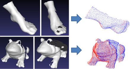
Fig. 6.9 Two views of Foot (top) and Frog (bottom). Separated views (left) and aligned views (right). The portion of overlap is large for both of the objects

Fig. 6.9 we show the two objects, the overlapping region of both of the objects in the two views is quite large (i.e. around 80 %). The Foot model has approximately 1500 points, while Frog is composed of around 5000 points for each view. The two views have been acquired separately by two scans and are already aligned by the authors of [79], as shown in Fig. 6.9 (right). In order to evaluate the robustness of pairwise registration methods against the initial pose variation, we define 30 poses by generating random angles sampled from a uniform distribution between 0◦ and 10◦ (for the three Euler’s angles) and random translations (for the three translation components tx , ty , tz ) such that the translation is 5 % of the object’s main diagonal. Indeed, such transformations are considered as ground truth. We evaluate the performance of three methods: (i) Besl’s ICP [7] (Besl), which is described in Sect. 6.2.2, (ii) Chen and Medioni ICP [23], (Chen) which introduces the point-to- plane distance, and (iii) Picky ICP proposed by Zinsser et al. [101] (Picky) which implements a combination of ICP variations described in Sect. 6.2.3. A hierarchical sampling strategy is introduced to improve the speed, and a thresholding approach on the residual distribution is employed. More specifically, a threshold is defined as TH = μ + 2.5σ , where μ = mean({ei }), and σ = std({ei }). According to the basic ICP algorithm described in Sect. 6.2.2, the threshold of Step 4 is set as 0.00001 but in most of the evaluated experiments the algorithm stops because it reaches the maximum number of iterations. Therefore, we define two settings with maximum number of iterations 15 and 50 respectively in order to evaluate the speed of convergence for the analyzed cases.

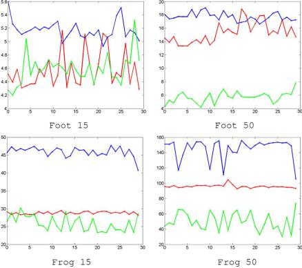
In Fig. 6.10, computational efficiency is evaluated. Experiments were carried out on an entry-level laptop at 1.66 Ghz with 4 Gb. The algorithms are coded using Matlab. The three methods are shown in red (Besl), blue (Chen), and green (Picky). In general, the best results were obtained by the Picky algo-

Fig. 6.10 Computational time evaluation. Time (sec) employed for each pairwise registration. The three methods are shown in red (Besl), blue (Chen), and green (Picky)

rithm. Moreover, due to the higher computational cost of the point-to-plane distance, the Chen method is the slowest. Note that a drastic reduction of registration speed is observed when the number of points increases from Foot to

Frog.

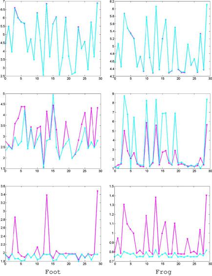
In Fig. 6.11, the accuracy of registration is evaluated. In general, especially when the ground truth is not available, a good accuracy evaluation criterion is the Mean Squared Error (MSE) (i.e. mean{ei }). Note that the MSE error is not comparable between the three methods since they compute different distance measures and, in Picky, the error generated by outliers is not considered. Note that, for both the objects, MSE error of Besl does not improve when the number of iterations increases. Conversely, in Picky, the benefit of a higher number of iterations is observed and most of the registrations are able to reach convergence.

In order to get a direct comparison between the methods we use the ground truth transformations, which are available since we have generated them. Indeed, we evaluate the rotation and the translation error, as shown in Figs. 6.12 and 6.13

Fig. 6.11 MSE evaluation for Besl (top), Chen (middle), and Picky (bottom). The cases employing 15 iterations are shown in magenta, while cases employing 30 iterations are shown in cyan

respectively. Rotation error is computed as the mean of the difference between the observed Euler’s angles of the estimated transform and the ground truth. Angles are in radians. Translation error is the norm of the difference between the two translation vectors.