Материал: [2.1] 3D Imaging, Analysis and Applications-Springer-Verlag London (2012)
240 |
U. Castellani and A. Bartoli |
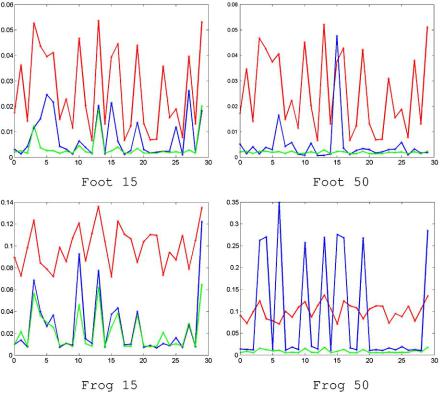
Fig. 6.12 Rotation error. The three methods are shown in red (Besl), blue (Chen), and green (Picky). Note that peaks correspond to failures of the pairwise registration procedure
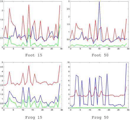
Table 6.1 summarizes the experiments by showing the mean of the evaluated measures. We observe better accuracy by using Picky. Note also that in general Chen outperforms Besl. Finally, we also show in Table 6.1 the number of failures (or divergences) because a local minimum is reached. We show that in more than half of the cases the convergence is reached within 15 iterations. Again the best results are shown with Picky since no failures are observed after 50 iterations and it always converges after 15 iterations with Foot. We observed also that the cases of failures of Besl and Chen methods are related to the strongest variations of starting pose, thus confirming the importance of a good initialization procedure.
6.5 Case Study 1: Pairwise Alignment with Outlier Rejection
In this section, we describe a simple but effective strategy to make the ICP algorithm resistant to incorrect correspondences. Particularly when views are only par-
6 3D Shape Registration |
241 |
Fig. 6.13 Translation error. The three methods are shown in red (Besl), blue (Chen), and green (Picky). Note that peaks correspond to failures of the pairwise registration procedure
tially overlapped, many points of the data-view do not have a correspondence in the model-view. We call those points single-points. However, the basic ICP algorithm enforces single points to be associated to closest points in the model-view, therefore generating outliers. A robust outlier rejection procedure is introduced based on the so-called X84 rule [17, 40]. The idea is to perform a robust statistical analysis of the residual errors ei after closest point computation. The underlying hypothesis was pointed out in [100] and consists of considering the residuals of two fully overlapping sets as an approximation of a Gaussian distribution. Non-overlapping points can be detected by estimating a Gaussian distribution from residual errors and by defining a threshold on the tails of the estimated Gaussian.
The X84 rule is a tool to automatically and robustly estimate this threshold. Given the set of residual errors, E = {ei }, i = 1 . . . Nd , the Median Absolute Deviation (MAD) is defined as:
MAD = med |ei − location| , |
(6.10) |

242 U. Castellani and A. Bartoli
Table 6.1 Summary of performance evaluation. The mean of the 30 pairwise registrations for each evaluated measure is shown
Exp. |
MSE error |
Rot. error |
Trans. error |
Number of |
Time |
|
(mm) |
(rad.) |
(mm) |
divergences |
(sec) |
|
|
|
|
|
|
Besl Foot 15 |
4.681 |
0.026 |
0.922 |
13/30 |
4.568 |
Chen Foot 15 |
3.155 |
0.007 |
0.593 |
15/30 |
5.173 |
Picky Foot 15 |
2.084 |
0.003 |
0.195 |
6/30 |
0.593 |
Besl Foot 50 |
4.672 |
0.025 |
0.853 |
13/30 |
15.309 |
Chen Foot 50 |
2.725 |
0.004 |
0.601 |
5/30 |
17.680 |
Picky Foot 50 |
1.910 |
0.001 |
0.104 |
0/30 |
5.683 |
Besl Frog 15 |
4.905 |
0.099 |
2.936 |
14/30 |
28.811 |
Chen Frog 15 |
2.203 |
0.026 |
0.976 |
10/30 |
45.917 |
Picky Frog 15 |
0.932 |
0.021 |
0.411 |
9/30 |
25.850 |
Besl Frog 50 |
4.906 |
0.099 |
2.939 |
5/30 |
95.882 |
Chen Frog 50 |
3.217 |
0.092 |
2.608 |
9/30 |
145.028 |
Picky Frog 50 |
0.765 |
0.008 |
0.069 |
0/30 |
50.292 |
|
|
|
|
|
|
where med is the median operator and location is the median of residual errors (i.e., med(E)). The X84 rule prescribes to reject values that violate the following relation:
|ei − location| < k · MAD. |
(6.11) |
Under the hypothesis of Gaussian distribution, a value of k = 5.2 is adequate in practice, as the resulting threshold contains more than 99.9 % of the distribution.
Now we are ready to define the new procedure for robust outlier rejection:
1.For all data-points di D, compute the error ei according to Eq. (6.4) (i.e. by estimating the closest point and by generating the pair of corresponding points ci = (di , mj )).
2.Estimate location by computing the median of residuals, med(E).
3.Compute MAD according to Eq. (6.10).
4.For each residual error ei (i = 1, . . . , Nd ):
a.If ei satisfies Eq. (6.11) then keep ci in the list of correspondences,
b.If not, reject the correspondence.
5.A new list of corresponding points cˆi is obtained from which outliers have been filtered out.
In practice, this procedure replaces step 1 in the ICP algorithm described in Sect. 6.2.2. The X84 rejection rule has a breakdown point of 50 %: any majority of the data can overrule any minority. The computational cost of X84 is dominated by the cost of the median, which is O(n), where n is the size of the data point set. The most costly procedure inside ICP is the establishment of point correspondences,
6 3D Shape Registration |
243 |
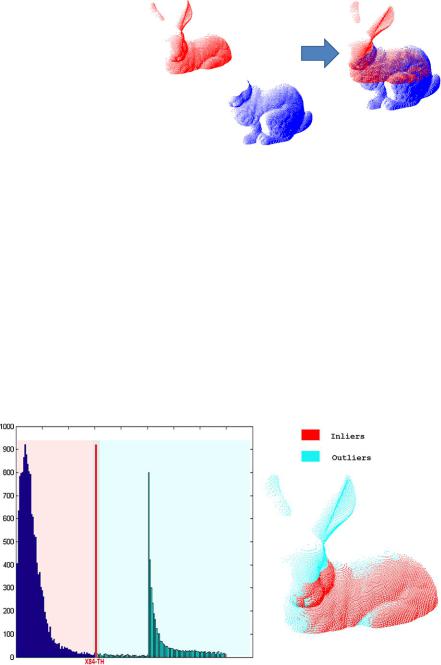
Fig. 6.14 Registration with robust outliers rejection. Two views at starting pose (left) and after registration (right). Note that the overlap area is quite restricted
which costs O(n log n). Therefore X84 does not increase the asymptotic complexity of ICP.
In Fig. 6.14, an example of registration between two views with a strong occluded part is shown. The non-overlapping area is wide: the ears and the whole face of Bunny are only visible in the data-view while the bottom part of the body is observed in the model-view only. The number of data points is Nd = 10000, the number of model points is Nm = 29150, and the number of points of the overlap is #(D ∩ M) = 4000. In this experiment, the two views are synthetically sampled from the whole 3D model. A view mask of 600 × 500 points is used in order to obtain highly dense views. Moreover, in this fashion, we know the ground truth transformation and no noise affects the views. Figure 6.15 shows the distribution of residual errors after X84-ICP registration. Note that most of the residuals are concentrated around zero. It is confirmed that the behavior of the early part of the distribution is similar to a Gaussian [100]. The X84 rule is employed and the threshold is automatically estimated on the tail of the Gaussian.
Fig. 6.15 Automatic residuals thresholding. From the distribution of residuals, the threshold is estimated according to the X84 rule. Points under the threshold are inliers (red), while outliers are over the threshold (blue). Outliers are points in non-overlapping areas

244 |
|
|
|
U. Castellani and A. Bartoli |
|
Table 6.2 X-84 performance evaluations. Rotation and translation errors are reported |
|
||||
|
|
|
|
|
|
Method |
Rot. error |
Trans. error |
Number of |
Number of |
Time |
|
(rad.) |
(mm) |
overlap. points |
iterations |
(sec) |
|
|
|
|
|
|
Besl |
0.22345 |
1.2636 |
10000 |
20 |
370 |
Picky |
0.10918 |
0.9985 |
9534 |
28 |
76 |
X84-ICP |
0.06351 |
0.4177 |
4582 |
21 |
383 |
Ground Truth |
– |
– |
4000 |
– |
– |
|
|
|
|
|
|
The second peak of the distribution corresponds to residuals generated by the nonoverlapping points.4 In Fig. 6.15 (right), points of the data-view are colored differently between inliers and outliers. Note that non-overlapping parts are correctly registered.
Table 6.2 summarizes the performance of X84-ICP in comparison with Besl and Picky. The ground truth transformation is shown as well. Note that the basic ICP is strongly affected by outliers and is not able to correctly align the two views. The Picky ICP improves the accuracy, but it is not able to correctly estimate the overlapping parts and it does not reach convergence. Conversely, by employing the X84 rule wrong correspondences are well detected and a correct registration is obtained. We highlight that although X84-ICP performs well in this experiment, in more general cases where the number of outliers is greater than 50 % of the residual distribution, the X84 rule is likely to fail.
6.6 Case Study 2: ICP with Levenberg-Marquardt
In this section, we describe a registration method called Levenberg-Marquardt ICP (LM-ICP), which addresses several of the issues of ICP by modeling the registration as a general optimization problem. LM-ICP [32] was proposed in order to minimize the alignment error by employing a nonlinear optimization procedure. The advantage of the LM-ICP is the versatility in the definition of the optimization function in order to take into account of several aspects of the registration, such as outlier rejection and speed.
6.6.1 The LM-ICP Method
The general problem formulation is defined as for the ICP algorithm. The error function E(a) = EICP(a, D, M) is Nonlinear Least Squares and can thus be written
4In order to visualize the peak the second part of the histogram has been quantized with wider intervals.