Материал: [2.1] 3D Imaging, Analysis and Applications-Springer-Verlag London (2012)

The final elevation error can be propagated from each variable presented in Eqs. (9.8), (9.14) and (9.15), as a function of H , B, α, r , and r (i.e. phase difference ψ ). Based on geometric errors caused by H , B, α, r , and ψ , the related elevation error can be calculated by partially differentiating these functions [126], as shown in Eq. (9.21).

δhH = δH

where τ is the terrain surface slope in the slant range direction. The overall elevation error can be a sum of the errors presented in Eq. (9.21). To rectify errors in Eqs. (9.21), a useful way to identify errors is from the following three aspects.

1.Random errors. These are errors randomly introduced in the DEM generation procedures, such as, electronic noise of SAR instruments and interferometric phase estimation error. They cannot be compensated by tie points, which are the corresponding points where their corrected ground positions are known. The random errors affect the precision of the InSAR system, while the following errors determine the elevation accuracy.

2.Geometric distortion. These include altitude errors, baseline errors, and SAR internal clock timing errors (or atmospheric delay). They are systematic errors that may be corrected by tie points.

3.Position errors. These errors include orbit errors and SAR processing azimuthlocation errors and may be removed by a simple vertical or horizontal shift in the topographical surface.

From the above discussion, it can be seen that the elevation accuracy of DEMs generated from InSAR is influenced by various factors. Atmospheric irregularities affect the quality of SAR images and induce errors in the interferogram phase. Terrain types also contribute to the accuracy as scattering composition and geometry. This can be seen from Eq. (9.21) where the terrain surface slope along the slant range direction makes contributions to a few original errors, such as the original baseline error and phase error. Theoretically the interferometric nature used in DEM generation from InSAR gives the height accuracy to the level of the SAR wavelength (i.e. millimeters to centimeters), which match the phase difference. However this is hard to achieve in practice due to the errors mentioned above and the uncertainty introduced by imaging geometry and atmospheric irregularities (especially for repeat-pass interferometry). It was reported that atmospheric effects on a repeatpass InSAR could induce significant variations in an interferogram of 0.3 to 2.3 phase cycles. For an ERS interferogram with a baseline of 100 m, elevation errors of up to about 100–200 m can be caused by the atmospheric effects on DEMs [70].

Quantitative validation of DEMs generated from InSAR needs ground truth for comparison, such as GCPs or DEMs generated by higher accuracy instruments. As with DEM generation from optical stereoscopic imagery, RMSE and standard deviation can be used as metrics in accuracy evaluation. Reported elevation accuracy for the SRTM7 data [82], created using C-band InSAR, was 2–25 m, with a significant variation depending on the terrain and ground cover types (i.e. vegetation). When vegetation is dense, InSAR does not provide good DEM results, while there is only sparse/low vegetation, the elevation accuracy can achieve 2 m. Horizontal resolution of SRTM SAR data is typically about 90 m for most areas, which is much worse than 2–20 m resolution of optical satellite images. ERS-1 and ERS-2 were exploited in DEM generation by Mora et al. [113], and the reconstructed DEMs were compared with those from SRTM InSAR in the same areas with maximum difference of 35–60 m and standard deviation of 3–11 m. Normally ±10 m elevation accuracy is expected from SRTM InSAR generated DEMs [123].

Due to difficulties in meeting the geometric requirement to the coherent conditions for two complex SAR images in interferometry, InSAR is not yet as popular as its counterpart of stereoscopic imagery in DEM generation [88]. In comparison with satellite stereoscopic imagery, the major advantage of InSAR is that it is independent from weather conditions—SAR illuminates its target with the emitted electromagnetic wave and the antenna receives the coherent radiation reflected from the target. In areas where optical sensors fail to provide data, such as heavy cloud areas, InSAR can be used as a complementary sensing mode for global DEM generation.

9.3.3 Examples of DEM Generation from InSAR

The first example presented in this section is a DEM from SRTM data [123]. The parameters of the interferometer are listed in Table 9.2.

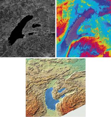
Figure 9.9 (top left) shows the magnitude (or amplitude) of SRTM raw data from the master antenna. The imaging area consists of 600 × 450 pixels. Each pixel of the image is a complex value of amplitude and phase as shown in Eq. (9.7). Figure 9.9 (top right) is the phase of the interferogram, and the reconstructed DEM is presented in Fig. 9.9 (bottom).

The processing of the SRTM InSAR data to the DEM is split into two parts: the InSAR data processing part and the geocoding part. The first part covers the steps necessary to get from the sensor raw data to the unwrapped phase, while the second part deals with precise geometric transformation from the sensor domain to map the cartographic coordinate space.

7SRTM: Shuttle Radar Topography Mission aimed to obtain DEMs on a near global scale from 56◦ S to 60◦N.

Fig. 9.9 InSAR generated DEM of Lake Ammer, Germany. Top left: Magnitude of raw data. Top right: Interferogram phase. Bottom: DEMs from phase. Figure courtesy of [123]

b.The irregular grid is interpolated to a corresponding regular grid.

c.Slant range images are converted into their regular grid equivalents. The mapped DEM is demonstrated in Fig. 9.9(bottom).

The reconstructed DEM has horizontal accuracy, relative vertical accuracy, and absolute vertical accuracy of 20 m, 6 m and 16 m with LE90, respectively.

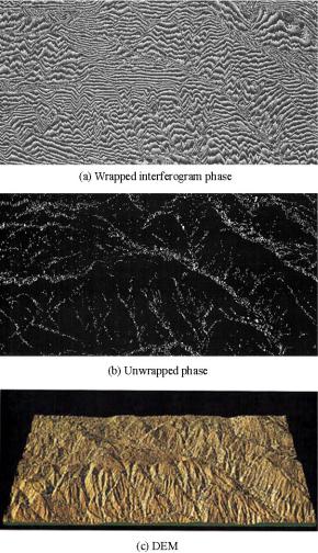
The second example is taken from a pair of ERS-1 SAR images of a mountainous region of Sardinia, Italy [37]. The image has 329 × 641 pixels. Figure 9.10(a) is the interferogram phase image, and Fig. 9.10(b) is the unwrapped phase image with the white points representing existing values. The phase unwrapping was done by a fast algorithm based on LS methods. It was claimed that the reconstructed DEM was in qualitative agreement with the elevation reported in geographic maps. Although the overall accuracy was not given because the published research was concentrated on the phase unwrapping algorithm, the computational time required for phase unwrapping process was achieved as 25 minutes on a Silicon Graphics Power Onyx RE2 machine for the mountainous region of Sardinia.

Fig. 9.10 InSAR generated DEMs from a pair of ERS-1 SAR images of a mountainous region of Sardinia, Italy. Figure courtesy of [37]

9.4 DEM Generation from LIDAR

9.4.1 LIDAR Data Acquisition

Airborne Laser Scanning (ALS) or LIght Detection And Ranging (LIDAR) has revolutionized topographic surveying for fast acquisition of high-resolution elevation data, which has enabled the development of highly accurate 3D products. LIDAR was developed by NASA in the 1970s [3]. Since the early 1990s, LIDAR has made significant contributions to many environmental, engineering and civil applications. It is being used increasingly by the public and commercial sectors [108] for forestry, archeology, 3D city map generation, flood simulations, coastal erosion monitoring,