Материал: [2.1] 3D Imaging, Analysis and Applications-Springer-Verlag London (2012)

•The orientation of the image is a combination of the platform heading due to orbital inclination, the yaw of the platform, and the convergence of the meridian.

•The scale factor in the along-track direction is a combination of the velocity, the altitude and the pitch of the platform, the detection signal time of the sensor and the component of the Earth’s rotation in the along-track direction.

•The leveling angle in the across-track direction is a combination of platform roll, the viewing angle, the orientation of the sensor and the Earth’s curvature.

Mathematical models establishing geometrical relationships between the image and cartographic coordinates can be rigorous or approximate [64]. Rigorous modeling can be applied when a comprehensive understanding of the imaging geometry exists. However in many cases, it is difficult to obtain accurate interior and exterior parameters of the imaging system due to the lack of sufficient control. Therefore, approximate modeling has been developed for real-world use. Approximate models include direct linear transformation (DLT), self-calibration DLT, rational function models, and parallel projection [64]. In analyzing the accuracy potential of DEMs generated by high-resolution satellite stereoscopic imagery, Fraser [48] pointed out that a mathematical model, such as collinearity equations, needs to be modified for different settings in a rigorous model with stereo-bundle adjustments, while in the absence of the sensors’ attitude data and sensors’ orbital parameters, approximate models are recommended.

To improve the imaging geometry, researchers have paid special attention to the B/H ratio in acquiring satellite stereo pairs. A systematic investigation was conducted by Hasegawa et al. [67]. In their research, the impact of the B/H ratio to DEM accuracy was analyzed and the conclusion was made that B/H ratios ranging from 0.5 to 0.9 give better results for automatic DEM generation from stereo pairs. Li et al. designed an accurate model of the intersection angle and B/H ratio for a spaceborne three linear array camera system [100]. It was indicated that the B/H ratio was directly related to the DEM accuracy. A favourable imaging geometry can be achieved by a B/H ratio of 0.8 or more [48]. With SPOT-5, the viewing angle can be adjusted to tune the across-track B/H ratio between 0.6 and 1.1 and the along-track B/H ratio to around 0.8 [150].

From an application point of view, errors of terrain representation (ETR) are also taken into account since these may propagate through GIS operations and affect the quality of final products which use DEMs [31]. When interpolation is needed, the way to represent the terrain surface contributes to DEM accuracy. Chen and Yue [31] developed a promising method of surface modeling based on the theorem of surface. In their work, a terrain surface was defined by the first and second fundamental coefficients with information of the surface geometric properties and its deviation from the tangent plane at the point under consideration. It was demonstrated in their work that a good criterion for DEM accuracy evaluation should have included not only errors generated in 3D reconstruction from stereoscopic geometry but also ETR at a global level. When using a DEM in an application product, ETR should be counted as an input error.

9.2.3 An Example of DEM Generation from SPOT-5 Imagery

In this section, the main steps in DEM generation from a satellite stereoscopic image pair are outlined. The example presented in this section is from [149]. The study site is the area around Quebec City, QC, Canada (47◦N, 71◦30 W). The information of the SPOT-5 stereo images in panchromatic mode is listed in Table 9.1.

A perspective projection model is established based on the geometric positions of the satellite, the camera, and the cartographic coordinate. This model links the 3D cartographic coordinate to the image coordinates, and the mathematical expression is given by Eqs. (9.3) and (9.4) [147, 148]:

where

Parameters involved in Eqs. (9.3)–(9.6) are explained as follows.

His the altitude of the point corrected for Earth curvature;

ais mainly a function of the rotation of the Earth;

αis the instantaneous field-of-view;

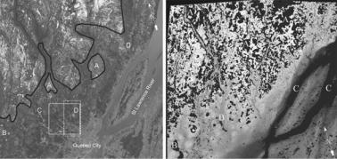
Fig. 9.4 Left: SPOT-5 image captured on 5 May 2003. Right: DEM generated from the stereo pair. A: melting snow; B: frozen lakes; C: the St. Lawrence River with significant melting ice; D: down-hill ski stations with snow. Figure courtesy of [149]

The ground control points (GCPs) with known (x, y, z) coordinates and corresponding (u, v) image coordinates are employed for the bundle adjustment to obtain parameters in the mathematical model. The processing steps of DEM generation from SPOT-5 stereo images (see Fig. 9.4(left)) are as follows.

1.Acquisition and pre-processing of the remote sensed data (images and metadata showing configuration of image acquisition) to determine an approximate value for each parameter of the 3D projection model.

2.Collection of GCPs with their 3D cartographic coordinates and 2D image coordinates. GCPs covered the total surface with points at the lowest and highest elevation to avoid extrapolations, both in x, y and elevation.

3.Computation of the 3D projection model, initialized with the approximate parameter values and refined by an iterative least-squares bundle adjustment with the GCPs.

4.Extraction of matching points from the two stereo images by using a multi-scale normalized cross-correlation method with computation of the maximum of the correlation coefficient.

5.Computation of (x, y, z) cartographic coordinates from the matching points in a regular grid spacing using the adjusted projection model (from step 3).

The full DEM (60 km × 60 km with a 5 m grid spacing) is extracted as shown in Fig. 9.4(right). It reproduces the terrain features, such as the St. Lawrence River and a large island in the middle. The black areas correspond to mismatched areas due to radiometric differences between the multi-date images. In this case, they are a result of snow in the mountains and on frozen lakes. The quantitative evaluation is conducted by comparison of the DEM generated from the SPOT-5 stereo images to a LIDAR acquired DEM with the accuracy of 0.15 m in elevation. Accuracies of 6.5 m (LE68) and 10 m (LE90) were achieved, corresponding to an image matching error of ±1 pixel.

9.3 DEM Generation from InSAR

Interferometric Synthetic Aperture Radar (InSAR) is the combination of SAR and interferometry techniques. SAR systems, operating at microwave frequencies, provide unique images representing the geometrical and electrical properties of the surface in nearly all weather conditions. DEM generation from InSAR is an active sensing process which is largely independent of weather conditions and can operate at any time throughout the day or night. A conventional SAR only produces 2D images reflecting the location of a target in the along-track axis, which is the axis along the flight track (azimuth range, X), and the across-track axis, which is the axis defined as the range from the SAR to the target (slant range, Y ). The altitudedependent distortion of SAR images can only be viewed in X and Y with ambiguous interpretation. Therefore, it is impossible to use a single SAR image to recover surface elevation. The development of InSAR techniques has enabled measurement of the third dimension (the elevation), which relies on the phase difference from two SAR images covering the same area and acquired from slightly different angles.

DEM generation from satellite-based SAR was reviewed by Toutin and Gray [151] with four different categories: stereoscopy, clinometry, polarimetry and interferometry (InSAR). Stereoscopy employs the same geometric triangulation principle used in optical stereoscopy for recovering elevation information, clinometry utilises the concept of shape from shading and polarimetry works on a complex scattering matrix based on a theoretical scattering model for tilted and slightly rough dielectric surfaces to calculate the azimuthal slopes, hence generating the elevation. InSAR also employs triangulation, but in a different implementation to stereoscopy, and can measure to an accuracy of millimeters to centimeters, which is a fraction of the SAR wavelength, whereas the other three methods are only accurate to the order of the SAR image resolution (several meters or more) [129]. DEM generation from InSAR is introduced in this section. For the other categories, please refer to [151] for details.

9.3.1 Techniques for DEM Generation from InSAR

The concept of incorporating interferometry to radar for topographic measurement can be traced back to Roger and Ingalls’ Venus research in 1969 [127]. Zisk used the same method for moon topography measurements [184], while Graham employed InSAR for Earth observation by an airborne SAR system [56]. However the real development of InSAR in DEM generation from spaceborne SAR instruments has been supported by the availability of suitable globally acquired SAR data from ERS-1 (1991), JERS-1 (1992), ERS-2 (1995), RADARSAT-1 (1995), SRTM (2000), Envisat (2002), RADARSAT-2 (2007), and TanDEM-X (2010). The technique has been considered mature since the late 1990s. The following section introduces InSAR concepts and their application to DEM generation.

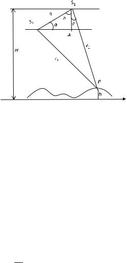
Fig. 9.5 InSAR imaging geometry: The radar signal is transmitted from antenna S1 and received simultaneously at S1 and S2. The phase difference of the two echoes is proportional to r , which depends on the baseline angle α, look angle θ , satellite altitude H , range vectors r1 and r2, and target elevation h

9.3.1.1 Basic Principle of InSAR in Elevation Measurement

InSAR in DEM generation requires that two SAR images of a target are acquired from different positions by a sensor (or sensors) with nearly the same observation angles. The phase difference between these two observations is then used to derive the elevation. The two SAR images can be taken at the same time (single-pass interferometry) or at different times (repeat-pass interferometry) over the target. Figure 9.5 depicts a simplified InSAR imaging geometry [1]. S1 and S2 are two sensor positions, r1 and r2 are range vectors from the two sensors to the target point P with elevation h, satellite altitude is H , the baseline is B, α is the baseline orientation

where A is the amplitude and φ is the phase. Two complex SAR images (a ‘master’ and a ‘slave’) are formed from positions S1 and S2. Therefore the phase difference ψ between S1 and S2 is directly related to the path difference between r1 and r2, as follows:

where λ is the SAR signal wavelength, and r = r2 − r1.

The imaging geometry in Fig. 9.5 demonstrates the relationship of B, r1, r2, α, and θ . In order to derive the formula which expresses the relationship quantitatively, two additional elements are introduced: one is point A, a perpendicular intersection point of line S1A and line S2A, and the other is angle β, the complementary angle of 90◦ to α in the right angled triangle S1S2A. According to a trigonometric theorem,