Материал: [2.1] 3D Imaging, Analysis and Applications-Springer-Verlag London (2012)

9 3D Digital Elevation Model Generation |
381 |
In the right angled triangle S1S2A of Fig. 9.5, sin β = cos α and cos β = sin α. Substituting these into the right-hand side of Eq. (9.10), we have
cos(β + θ ) = sin α cos θ − cos α sin θ = − sin(θ − α) |
(9.11) |
Substituting Eq. (9.11) to Eq. (9.9), the relationship of B, r1, r2, α, and θ is expressed in Eq. (9.12), and the target elevation h can be calculated from Eq. (9.13) based on the geometric relation shown in Fig. 9.5.
|
− |
|
= |
r22 |
2r1B |
2 |
|
sin(θ |
|
α) |
|
− r12 − B |
(9.12) |
||
|
= H − r1 cos θ |
|
|||||
|
|
h |
|
(9.13) |
|||
In Eq. (9.12), r1 is replaced by r , and r2 by r + r , then it can be re-written as
sin(θ |
− |
α) |
= |
(r + r)2 − r2 − B2 |
(9.14) |
|
2rB |
||||||
|
|
|
Replacing cos θ in Eq. (9.13) by sin(θ − α) in such a way that it can be rewritten as
|
cos α 1 − |
|
sin2 |
|
− sin α sin(θ − α) |
|
h = H − r |
|
(θ − α) |
(9.15) |
In practice, the SAR altitude H , the baseline B, and the baseline orientation angle α are estimated from knowledge of the orbit, and the range r , half the roundtrip distance of radar signal, is measured by the SAR internal clock. Knowing the phase difference ψ from the interferometric fringes of two SAR images, the path difference r can be calculated from Eq. (9.8), hence sin(θ − α) can be derived from Eq. (9.14), and finally the elevation value is calculated from Eq. (9.15).
The phase difference between the two SAR images is normally represented as an interferogram, an image which is the product of the complex master image convolved with the complex slave image. It is important to appreciate that only the principal values of the phase, (i.e. modulo 2π ), can be measured from the interferogram. The 2π phase difference corresponds to one cycle of interferometric fringe. The total path difference of the two receivers is multiples of the radar wavelength, (i.e. multiples of 2π in terms of phase). The process of phase unwrapping estimates this integer number in the interferometry. It is a key process in DEM generation from InSAR.
In many cases, the InSAR imaging geometry may differ from that demonstrated in Fig. 9.5. However, the principle of deriving the target elevation from the interferogram is similar and involves the following two steps:
1.Find out the path difference from the phase difference.
2.Calculate the topography based on the path difference with other known geometric parameters.
Figure 9.5 is a simplified model and the phase of SAR signals contains other information beyond topography. For a detailed description of InSAR and a better understanding of the signal modeling, please refer to [72].
382 |
H. Wei and M. Bartels |
Fig. 9.6 Processing stages of DEM generation from InSAR
9.3.1.2 Processing Stages of DEM Generation from InSAR
DEM generation from InSAR may involve different approaches, as presented in various published work [1, 38, 71, 95, 123, 135, 180]. In general, the processing stages to generate DEMs from spaceborne InSAR can be summarized in Fig. 9.6.
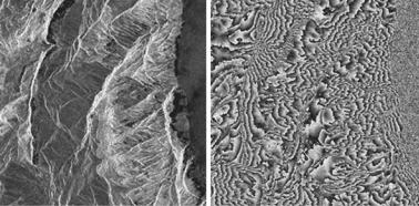
When two radar signals are acquired, image registration is accomplished either based on cross-correlation of the image radiometry (speckle correlation) or by optimizing phase patterns for the area extracted from the two images. All image registration techniques developed in the image processing community can be used for this purpose [185]. Visual identification of a corresponding point in both images sometimes is needed. Sub-pixel registration accuracy has been reported in the remote sensing community for InSAR image registration [102]. For those co-registered pixels, an interferogram is formed by averaging the corresponding amplitudes and differencing the corresponding phase at each pixel. The phase of the interferogram contains information on the differential range from the target to the SAR antenna in the two paths, which is related to the elevation of the target. Normally the interferogram needs to be filtered for noise removal. Many algorithms have been developed for interferogram filtering, such as filtering based on pivoting median [97], adaptive phase noise [86], locally adaptive [173], and adaptive contoured window approaches [178]. In case of the presence of large co-registration errors, various techniques can be used for error correction to ensure a high quality interferogram [99]. Figure 9.7 shows an example of interferogram images in the form of magnitude (left) and phase (right).
As mentioned previously, the interferogram phase shown in Fig. 9.7(right) only reflects the principal value of modulo 2π . The phase difference that corresponds to the path difference of the two SAR positions to a target, is a multiple of the 2π in terms of phase. The phase unwrapping process aims to recover the integer number, which gives the multiple of modulo 2π . InSAR phase unwrapping has remained an active research area for several decades. Many approaches have been proposed and applied. In their pioneering research, Goldstein et al. [54] proposed the integration of a branch-cut approach in 2D phase-unwrapping. Least squares methods for phase unwrapping were developed in 1970s [49, 79] and have been widely adapted in InSAR elevation estimation [71, 121]. In the last two decades, further methods have been developed including network programming [36], region growing [174], hierarchical network flow [29], data fusion by means of Kalman filtering [103], multichannel phase unwrapping with graph cuts [42], complex-valued Markov random field
9 3D Digital Elevation Model Generation |
383 |
Fig. 9.7 Interferogram images from InSAR. Left: magnitude. Right: phase. The original two SAR images are ERS-1 data, imaging Sardinia, Italy, from frame 801, orbit 241, August 2, 1991 and orbit 327, August 8, 1991, centered at 40◦ 8 N, 9◦ 32 E. 512× 512 pixels represent a 16 km × 16 km portion of the scene. Figure courtesy of http://sar.ece.ubc.ca/papers/UNWRAPPING/PU.html
model [176], particle filtering [110], phase unwrapping by Markov chain Monte Carlo energy minimization [5], and cluster-analysis-based multi-baseline phase unwrapping [177].
Fundamentally all existing phase unwrapping algorithms start from the fact that it is possible to determine the discrete derivatives of the unwrapped phase, that are the neighbouring pixel differences in the wrapped phase when these differences are mapped into the interval of (−π, π ). By summing these discrete derivatives (or phase differences), the unwrapped phase can be calculated. This is based on the assumption that the original scene is sampled densely enough and the true (unwrapped) phase does not change by more than ±π between adjacent pixels. If the hypothesis fails, so-called phase inconsistencies occur, that can lead to phase unwrapping errors. Phase unwrapping algorithms differ in the way that they deal with the difficulty of phase inconsistencies. Two classical approaches to phase unwrapping, branch cuts and least squares, are now detailed [129].
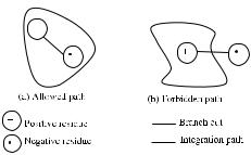
The Branch-Cut Method of Phase Unwrapping The basic idea is to unwrap the phase by choosing only paths of integration that lead to self-consistent solutions [54]. Theoretically the unwrapped solution should be independent of the integration path. This implies that the integral of the differenced phase of a closed path is zero in the error-free case. In other words, phase inconsistencies occur when the phase difference summed around a closed path formed by each mutually neighbouring set of four pixels is non-zero. Referred as residues, these points are classified as either positively or negatively ‘charged’ depending on the sign of the sum in a clockwise path. Branch-cuts connect nearby positive and negative residues such that no net residues can be encircled and no global errors can be accumulated. Figure 9.8 illustrates an example of a branch cut and allowable and forbidden paths of integration.
384 |
H. Wei and M. Bartels |
Fig. 9.8 Integration paths in phase unwrapping under the branch-cut rule
One key issue in the design of branch cuts based unwrapping algorithms is the selection of optimum cuts, especially when the density of the residue population is high. The algorithm developed by Goldstein et al. [54] gives the following steps to connect residues with branch cuts.
1.The interferogram is scanned until a residue is found.
2.A box of size 3 × 3 pixels is placed around the residue and is searched for another residue.
3.If found, a cut is placed between them.
•If the sign of the two residue is opposite, the cut is designated ‘uncharged’ and the scan continues for another residue.
•If the sign of the residue is the same as the original, the box is moved to the new residue and the search continues until either an opposite sign residue is located or no new residues can be found within the boxes.
4.For the latter case in step 3, the size of the box is increased by 2 pixels and the algorithm repeats from the current starting residue.
Finally, all of the residues lie on cuts that are uncharged, allowing no global error. The phase differences are integrated in such a way that there is no integration path crossing any of the cuts. Although branch-cuts based algorithms provide an effective way in phase unwrapping, the main disadvantage is that it may need operator intervention to succeed [44].
The Least Squares (LS) Method of Phase Unwrapping LS algorithms minimize the mean square difference between the gradients of the unwrapped phase (estimated solution) and the wrapped phase. Ghiglia and Romero gave the following expression for the sum t to be minimized [53]:
M−2 N −1 |
φi+1,j − φi,j − i,jx |
|
2 |
M−1 N −2 |
φi,j +1 − φi,j − i,jy |
|
2 |
(9.16) |
t = |
|
+ |
|
|||||
|
|
|
|
|
|
|
||
i=0 j =0 |
|
|
|
i=0 j =0 |
|
|
|
|
where φi,j is the unwrapped estimate corresponding to the wrapped value ϕi,j and:
i,jx |
= W (ϕi,j − ϕi−1,j ) |
(9.17) |
i,jy |
= W (ϕi,j − ϕi,j −1) |
|
9 3D Digital Elevation Model Generation |
385 |
with the operator W () wrapping values into the range of −π ≤ ϕ ≤ π . M and N refer to the image size in two dimensions. To find the minimum in Eq. (9.16) is equivalent to solving the following system of linear equations:
(φi+1,j − 2φi,j + φi−1,j ) + (φi,j +1 − 2φi,j + φi,j −1) = ρi,j |
(9.18) |
||
where |
|
. |
|
ρi,j = i,jx − ix−1,j + i,jy − i,jy |
−1 |
(9.19) |
|
Equation (9.18) represents a discretized version of Poisson’s equation [121]. The LS problem can be formulated as the solution of the set of linear equations:
Aφ = ρ |
(9.20) |
where A is an MN × MN sparse matrix, vector ρ contains values of wrapped phase, and vectors φ is the unwrapped values to be estimated. Although LS based methods are computationally very efficient when they make use of Fast Fourier transform (FFT) techniques, they are not very accurate because local errors tend to spread without means of limitation [53].
In practice, it is hard to operate the phase unwrapping process in a totally automated fashion in spite of vast investigation and research in this aspect of InSAR [151]. Human interventions are always needed. Therefore, in order to improve automation, phase unwrapping remains an active research area.
9.3.2 Accuracy Analysis of DEMs Generated from InSAR
The accuracy of the final DEMs generated from InSAR may be affected by many factors from SAR instrument design to image analysis. The major problems can be summarized as follows [1].
1.Inaccurate knowledge of acquisition geometry.
2.Atmospheric or ionospheric delays.
3.Phase unwrapping errors.
4.Decorrelation on land use types (scattering composition or geometry) which increases phase noise in the interferogram.
5.Layover or shadowing, which may directly affect interferometry.
For InSAR operational conditions, a critical baseline was defined for choosing SAR image pairs to generate an interferogram [112]. The concept of the critical baseline was introduced to describe the maximum separation of the satellite orbits in the direction orthogonal to both the along-track (azimuth) and the across-track (slant). If the critical value is exceeded, it would not be expected to have clear phase fringes in the interferogram. Toutin and Gray [151] indicated that the optimum baseline is terrain dependent; moderate to large slopes can generate a phase that can be difficult to process in the phase unwrapping stage and a baseline between a third and a half of the critical baseline is good for DEM generation, if terrain slope is moderate.