Материал: Scientific Herald of the Voronezh State University of Architecture and Civil Engineering

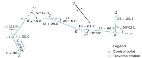
Fig. 2. Example of an open traverse [after Ghilani & Wolf, 2012]

One can extract three types of computational traverses as follow: 1 –– Closed polygon traverse.

2 –– Closed linked traverse.

3 –– Open traverse.

The first two types of computational traverse can be checked mathematically and can be adjusted due to the existence of conditions. The third type can not be checked or adjusted but only can be plotted.

2. Traverse Computations

In closed polygon traverse the minimum known parameters are: 1 –– Correct coordinates of a point.

2 –– Correct direction of a side (it is better if the known point lays on it). 3 –– Observed angles between sides.

4 –– Observed side lengths.

One can abstract general computations steps as follow:

Step 1: Computation of angles misclosure. Step 2: Balancing angles.

Step 3: Computation of preliminary directions. Step 4: Computation of departures and latitudes. Step 5: Computation of linear misclosure.

Step 6: Traverse adjustment.

Step 7: Computation of final coordinates.

The correct sum of internal angles can be computed as follow:

41

Scientific Herald of the Voronezh State University of Architecture and Civil Engineering. Construction and Architecture

In order to compute the angles misclosure one need to compute the sum of observed angles ∑\. Then the angles misclosure can be computed as follows:

The permissible angles misclosure C in seconds can be computed as follows:

Where: n is the number of observed angles and K is a constant depend on the level of traverse accuracy. According to Federal Geodetic Control Subcommittee (FGCS) K takes the following values:

First-order class I = 1.7" Second-order class I=3" Second-order class II=4.5" Third-order class I=10" Third order class II=12"

There are two methods of balancing angles [Ghilani & Wolf, 2012]:

1 –– Applying an average correction to each angle where observing conditions were approximately the same at all stations. The correction for each angle is found by dividing the total angular misclosure by the number of angles.

2 –– Making larger corrections to angles where poor observing conditions were found.

The first method is widely used because of the lack of knowledge related to observation conditions.

The preliminary whole circle bearings (WCB) can be computed as follows:

The angle in between is positive if it was observed clockwise and it will be negative if it was observed anticlockwise.

The departure and latitude of sides of the traverse can be computed as follows:

Departure misclosure is the algebraic sum of all traverse departures and the same for latitude misclosure. So the linear misclosure can be computed as follows:

42

The relative precision can be computed as:

Traverse adjustment can be carried out by computing the corrections of both departure and latitude of any side AB using the following equation:

Then the adjusted departure and latitude can be obtained by adding the corrections to the computed departures and latitudes.

The final coordinates can be computed as follow:

3. Closed Linked Traverse

In closed linked traverse the minimum known parameters are:

1 –– Correct coordinates of both starting and ending points of the traverse.

2 –– Correct directions of both starting and ending sides (the starting and ending known points lays on them).

3 –– Observed angles between sides.

4 –– Observed side lengths.

One can abstract general computations steps as follow:

Step 1: Computation of directional misclosure. Step 2: Balancing directions accumulatively.

Step 3: Link stating and ending points to form a virtual polygon. Step 4: Computation of departures and latitudes.

Step 5: Computation of linear misclosure.

Step 6: Traverse adjustment excluding the linking side. Step 7: Computation of final coordinates.

The directional misclosure can be computed by using equation (5) starting with the first known WBC and the observed angles between traverse sides until reaching the ending known side. One can compute directional misclosure by comparing the computed WCB and the known WCB of the ending side.

43

Scientific Herald of the Voronezh State University of Architecture and Civil Engineering. Construction and Architecture

The balancing values can be obtained accumulatively using the equation:

Where:

i is the directional correction of side order i, n is the order of the ending traverse side.

The rest steps of closed linked traverse are similar to the steps of closed polygon traverse except that the linking side does not take any correction in departure and latitude because they are correct values.

4. Open Traverse

Open traverse can only be plotted using starting known point and the observed lengths and the observed angles. There is no adjustment can be carried out for this type of traverses and so one can avoid forming this type in surveying projects.

5. TravCAD Development

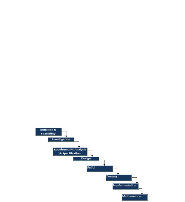
In order to achieve the research objective SW development life cycle using the water fall software model was adopted as shown in Figure 3.

Fig. 3. SW development life cycle using water fall model

Initiation & Feasibility: one can review current systems to see how to improve if possible. One did a feasibility study on the current systems to see if making a new system is feasible or not. By the end of the study one should have a project plan for the future stages of the cycle.

Investigation: one have to do a detailed investigation of the users needs, so one knows how the system will work. From this investigation one also is able to identify the inputs, processes, outputs and data flows by using all the information got from the current systems.

Requirement, analysis and specification: one must gather up all the information and plan out what the TravCAD system will be able to do.

44

Design: This stage helps to identify how the TravCAD system will look and run in details such as the interface design and coding.

Build: the developer use the plan that the design stage made and basically convert the information they got into computer code. Computer programs were written for every part of the system, normally done as series of modules in the project.

Testing: In this stage one used the test plans that should have been created in the design stage to test the system, so a check were carried out. A real life data were used to insure the reliability of the TravCAD.

Implementation: one needs to make sure that it has very few or no problems for system users. When the system is being installed the users will then be trained in how to use the new system. Maintenance: This is the final step in the cycle. Users of the developed system can report bugs they are dealt with. Some improvements can be applied on the system or the cycle can be returned to the first stage according to the conclusions and reports.

TravCAD SW was developed using VB6 programming language. It consists in this version of the following forms:

1 –– Starting form: Contains author affiliation and institution as shown in Figure 4.

Fig. 4. Starting Form

2 –– Identification form: identify SW name and purpose as shown in Figure 5.

Fig. 5. Identification Form

45