Материал: Маслов ИНТРОДУЦТИОН ТО ПХЫСИЦС ОФ СЕЦОНД-ОРДЕР МАГНЕТИЦ 2015

and one can see that F( x ,T ) < F(− x ,T ), thus the state with x > 0 , i.e., with the magnetic moments aligned along magnetic field, is more favorable than the state with x < 0 , i.e., with the magnetic moments

aligned against magnetic field. So, the state with x = − x < 0 is the local

minimum. Therefore the magnetic field removes the degeneracy. And what happens in the real systems at H = 0 ? In the real systems the only one of the two different macroscopic states ( M > 0 or M < 0 ) is realized. What is it? It turns out that under cooling the paramagnet to T = θ

the “random” selection of the state with x = x or with x = − x occurs.

And this choice depending on many random factors is made by Nature. In terms of the degree of degeneracy at T > θ we have one

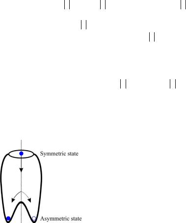
(nondegenerate) state ( x = 0 ), and at T < θ we have two states ( x > 0 and x < 0 ) with the same energies, i.e., doubly degenerated state (see Fig. 18.1).

Fig. 18.1. The variant

of “two-dimensional bottle”: the ball falls to one of the wells

In terms of symmetry, what do we mean by symmetric and asymmetric states when we talk about the system of magnetic moments. At

T > θ, M = 0 , thus the magnetization does not change the sign at replacing the selected axis z → −z . This is the symmetric state. At T < θ, magnetization M ≠ 0 , thus the magnetization changes the sign at replacing the selected axis z → −z . This is the asymmetric state. In this case the preferred direction occurs. Therefore at the paramagneticferromagnetic transition M = 0 → M ≠ 0 the spontaneous symmetry

46

breaking takes place. Note that in real solids the preferred orientations, so called easy magnetization axes, are always presented. On these axes the magnetization M is oriented at T < θ.

Let us look at this issue from the other side. Let us calculate σkz ,

where k is the number of arbitrary magnetic moment, without the meanfield approximation in the Ising model at H = 0

of N numbers σ1z ,σ2z ,...,σNz = ±1. Divide this sum on pairs of summands which differ in their signs. For example, one of these configura-

tions and the paired configuration will be

T. This is in contrast with our previous result (which is obtained in the mean-field approximation) and with the experiment. The reason is the availability of two degenerated states with the different orientation of

47

states are equal, so the probabilities of their realization are P1 = P2 = 12 .

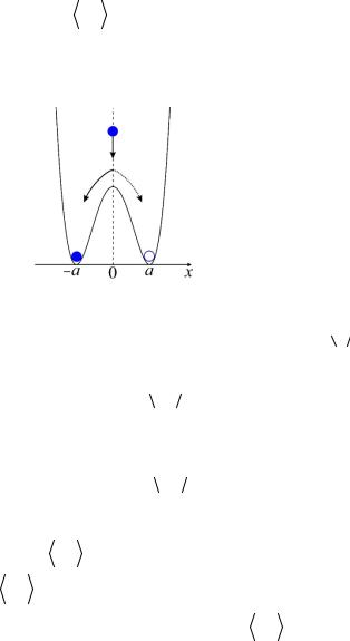
do not consider that at phase transition system “selects” one of the two states rather than it is located at both of them simultaneously. We can draw an analogy with the “two-dimensional bottle” (see Fig. 18.2).

Fig. 18.2. “Two-dimensional bottle” again

The probability that the ball will fall to the left or to the right minimum is equal to 12 . But the “mean coordinate” is x = −a 12 + a 12 = 0

which can not be.

So, calculating the σkz we took the mean values for all configura-

tions, half of which corresponds to σkz = +1 and the other one corresponds to σkz = −1, and the energies of these configurations are the

same at H = 0 . Thus, σkz h=0 = 0 . On the other hand, if H ≠ 0 , then

the degeneracy is removed, and the configuration with the magnetic moments aligned along the z-axis becomes more favorable. While calcu-

48

supposed that σkz ≠ 0 . This is the analogy to the magnetic field re-

moving the degeneracy.

Finally, at T < θ the order parameter x ≠ 0 (i.e., the magnetization is nonzero as well). But we can not determine the sign of the order parameter (or magnetization) beforehand, it is fully random.

19. Phenomenological Landau theory of second-order phase transitions

Let us discuss this theory briefly. In the previous paragraphs we developed the microscopic theory of phase transitions into ferromagnetic state, i.e., we took into account the real interactions between the magnetic moments (exchange interaction) and obtained the equation for the order parameter x , which was valid in the whole range 0 ≤ x ≤1 (in

other words at temperatures 0 ≤T ≤ θ and T > θ). We made this in the mean-field approximation. Also we found the Helmholtz free energy

function F (x,T ) in the whole range 0 ≤ x ≤1 and derived F (x,T ) at T near θ, i.e., x 1 . If we do not know the general form of F (x,T ) from the microscopic theory, we can not expand into series F (x,T ) at

x 1 , i.e., at T = θ.

Lev Landau did not know the microscopic theory of any secondorder phase transition known in the middle of XX century. He suggested that for all second-order phase transitions the Helmholtz free energy dependence on the corresponding order parameter ∆ (different for various second-order phase transitions) possessed the same form. But this

universal form function F (∆,T ) possessed only at small ∆ , i.e., near the critical temperature TC (for ferromagnetic transition we denoted it

θ). So, ∆ = 0 at T >TC , and ∆ 1 at T <TC , T →TC− , and ∆ further increasing as T decreases. At H = 0 this universal form is the following

49

where F0 (T ) is the component of free energy that is not related to the

effects of ordering. Actually this is the series expansion in powers of ∆ .

But the powers of ∆ and ∆3 are absent in this expansion, due to the fact that for all second-order phase transitions states with ∆ and −∆ are degenerated. And what are the parameters A and B? The experimental

series in powers of (T −TC ) considering only the first nonzero terms.

In the case of ferromagnetic transition we earlier obtained a =12 and b = 12θ . For the other second-order phase transitions these parameters

will be different. If the microscopic theory is absent then these coefficients are unknown. Nevertheless, we can obtain or estimate them from numerical calculations or from the experimental data.

2∆ a(T −TC )+ 2b∆2 = 0.

50