Материал: [2.1] 3D Imaging, Analysis and Applications-Springer-Verlag London (2012)
1 Introduction |
7 |
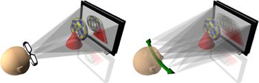
Fig. 1.2 Left: Stereoscopic displays use glasses-based polarization light separators to produce the two images required for stereoscopic reception. Right: Lens-based auto-stereoscopic displays project multiple, slightly displaced images by use of lenses or parallax barrier systems, allowing glasses-free stereoscopic reception. Such systems allow for slight head motion
to be recorded simultaneously. Typical displays require 8 to 28 simultaneous views and it is not feasible to record all views directly, because the amount of data would grow enormously. Also, the design of such multi-ocular cameras is difficult and expensive. Instead, a true 3D movie format is needed that allows us to synthesize the required views from a generic 3D image format. Currently, 3D data formats like Multi-View Depth (MVD) or Layered Depth Video (LDV) are under discussion [3]. MVD and LDV record both depth and color from few camera positions that capture the desired angular sections in front of the display. The many views needed to drive the display are then rendered by depth-compensated interpolation from the recorded data. Thus, a true 3D format will greatly facilitate data capture for future 3D-TV systems.
There is another obstacle to binocular perception that was not discussed in early binocular display systems. The observed disparity is produced on the image plane and both eyes of the human observer are accommodating their focus on the display plane. However, the binocular depth cue causes the eyes to physically converge towards the virtual 3D position of the object, which may be before or behind the display plane. Both, eye accommodation and eye convergence angle, are strong depth cues to our visual system and depth is inferred from both. In the real world, both cues coincide since the eyes focus and converge towards the same real object position. On a binocular display, the eyes always accommodate towards the display, while the convergence angle varies with depth. This conflict causes visual discomfort and is a major source of headaches when watching strong depth effects, especially in front of the screen. Stereographers nowadays take great care to balance these effects during recording. The only remedy to this disturbing effect is to build volumetric displays where the image is truly formed in 3D space rather than on the 2D display. In this case, the convergence and accommodation cues coincide and yield stress-free stereoscopic viewing. There is an active research community underway developing volumetric or holographic displays, that rely either on spatial pattern interference, on volume-sweeping surfaces, or on 3D lightfields. Blundell and Schwarz give a good classification of volumetric displays and sketch current trends [7]. All these 3D displays need some kind of 3D scene representation and binocular imaging is not sufficient. Hence, these displays also are in need of true 3D data formats.

8 |
R. Koch et al. |
1.3 The Development of Computer Vision
Although the content of this book derives from a number of research fields, the field of computer vision is the most relevant large-scale research area. It is a diverse field that integrates ideas and methods from a variety of pre-existing and coexisting areas, such as: image processing, statistics, pattern recognition, geometry, photogrammetry, optimization, scientific computing, computer graphics and many others. In the 1960s–1980s, Artificial Intelligence was the driving field that tried to exploit computers for understanding the world that, in various ways, corresponded to how humans understand it. This included the interpretation of 3D scenes from images and videos.
The process of scene understanding was thought of as a hierarchy of vision levels, similar to visual perception, with three main levels [38], as follows:
Low-level vision: early 2D vision processes, such as filtering and extraction of local image structures.
Mid-level vision: processes such as segmentation, generation of 2.5D depth, optical flow computation and extraction of regional structures.
High-level vision: semantic interpretation of segments, object recognition and global 3D scene reasoning.
This general approach is still valid, but it was not successful at the first attempt, because researchers underestimated the difficulties of the first two steps and tried to directly handle high-level vision reasoning. In his recent textbook Computer Vision: Algorithms and Applications [49], Rick Szeliski reports an assignment of Marvin Minsky, MIT, to a group of students to develop a computer vision program that could reason about image content:
According to one well-known story, in 1966, Marvin Minsky at MIT asked his undergraduate student Gerald Jay Sussman to “spend the summer linking a camera to a computer and getting the computer to describe what it saw”.15
Soon, it became clear that Minsky underestimated this challenge. However, the attempts to resolve the various problems of the three levels proved fruitful to the field of computer vision and very many approaches to solve partial problems on all levels have appeared. Although some vision researchers follow the path of cognitive vision that is inspired by the working of the human brain, most techniques today are driven by engineering demands to extract relevant information from the images.
Computer vision developed roughly along the above-mentioned three levels of vision. Research in low-level vision has deepened the understanding of local image structures. Digital images can be described without regard of scanning resolution by the image scale space [55] and image pyramids [50]. Image content can be described in the image domain or equivalently in the frequency (Fourier) domain, leading to a theory of filter design to improve the image quality and to reduce noise. Local
15Szeliski, Computer Vision: Algorithms and Applications, p. 10 [49].

1 Introduction |
9 |
structures are defined by their intrinsic dimension16 [4], which leads to interest operators [20] and to feature descriptors [6].
Regional relations between local features in an image or between images are powerful descriptions for mid-level vision processes, such as segmentation, depth estimation and optical flow estimation. Marr [38] coined the term 2.5D model, meaning that information about scene depth for a certain region in an image exists, but only viewed from a single view point. Such is the case for range estimation techniques, which includes stereo, active triangulation or time-of-flight depth measurement devices, where not a full 3D description is measured but a range image d (u, v) with one distance value per image pixel. This range value, along with some intrinsic parameters of the range sensing device, allows us to invert the image projection and to reconstruct scene surfaces. Full 3D depth can be reconstructed from multiview range images if suitably fused from different viewpoints.
The special branch of computer vision that deals with viewing a scene from two or more viewpoints and extracting a 3D representation of the geometry of the imaged scene is termed geometric computer vision. Here, the camera can be thought of as a measurement device. Geometric computer vision developed rapidly in the 1990s and 2000s and was influenced strongly by geodesy and photogrammetry. In fact, those disciplines are converging. Many of the techniques well known in photogrammetry have found their way into computer vision algorithms. Most notably is the method of bundle adjustment for optimally and simultaneously estimating camera parameters and 3D point estimates from uncertain image features [51].
Combining the geometric properties of scene objects with image based reflectance measurements allows us to model the visual-geometric appearance of scenes. There is now a strong relationship between computer vision and computer graphics that developed during the last decade. While computer graphics displays computer-defined objects with given surface properties by projecting them into a synthetic camera, vision estimates the surface properties of real objects as seen by a real camera. Hence, vision can be viewed as the inverse problem of graphics. One of the key challenges in computer vision is that, due to the projection of the objects into the camera, the range information is lost and needs to be recovered. This makes the inverse problem of recovering depth from images especially hard and often ill-posed. Today, both disciplines are still converging, for example in the area of image-based rendering in computer graphics and by exploiting the computing capabilities of Graphics Processing Units for computer vision tasks.
High-level vision attempts to interpret the observed scene and to assign semantic meaning to scene regions. Much progress has been made recently in this field, starting with simple object detection to object recognition, ranging from individual objects to object categories. Machine learning is vital for these approaches to work reliably and has been exploited extensively in computer vision over the last decade [43]. The availability of huge amounts of labeled training data from databases and the Web, and advances in high-dimensional learning techniques, are keys to the success
16Intrinsic Image Dimension (IID) describes the local change in the image. Constant image: 0D, linear structures: 1D, point structures: 2D.

10 |
R. Koch et al. |
of machine learning techniques. Successful applications range from face detection, face recognition and biometrics, to visual image retrieval and scene object categorization, to human action and event analysis. The merging of machine learning with computer vision algorithms is a very promising ongoing development and will continue to solve vision problems in the future, converging towards the ultimate goal of visual scene understanding. From a practical point of view, this will broaden the range of applications from highly controlled scenes, which is often the necessary context for the required performance in terms of accuracy and reliability, to natural, uncontrolled, real-world scenes with all of their inherent variability.
1.3.1 Further Reading in Computer Vision
Computer vision has matured over the last 50 years into a very broad and diverse field and this book does not attempt to cover that field comprehensively. However, there are some very good textbooks available that span both individual areas as well as the complete range of computer vision. An early book on this topic is the above-mentioned text by David Marr: Vision. A Computational Investigation into the Human Representation and Processing of Visual Information [38]; this is one of the forerunners of computer vision concepts and could be used as a historical reference. A recent and very comprehensive text book is the work by Rick Szeliski:
Computer Vision: Algorithms and Applications [49]. This work is exceptional as it covers not only the broad field of computer vision in detail, but also gives a wealth of algorithms, mathematical methods, practical examples, an extensive bibliography and references to many vision benchmarks and datasets. The introduction gives an in-depth overview of the field and of recent trends.17 If the reader is interested in a detailed analysis of geometric computer vision and projective multi-view geometry, we refer to the standard book Multiple View Geometry in Computer Vision by Richard Hartley and Andrew Zisserman[21]. Here, most of the relevant geometrical algorithms as well as the necessary mathematical foundations are discussed in detail. Other textbooks that cover the computer vision theme at large are Computer Vision: a modern approach [16], Introductory Techniques for 3-D Computer Vision [52], or An Invitation to 3D Vision: From Images to Models [36].
1.4 Acquisition Techniques for 3D Imaging
The challenge of 3D imaging is to recover the distance information that is lost during projection into a camera, with the highest possible accuracy and reliability, for every pixel of the image. We define a range image as an image where each pixel stores the distance between the imaging sensor (for example a 3D range camera)
17A pdf version is also available for personal use on the website http://szeliski.org/Book/.

1 Introduction |
11 |
and the observed surface point. Here we can differentiate between passive and active methods for range imaging, which will be discussed in detail in Chap. 2 and Chap. 3 respectively.
1.4.1 Passive 3D Imaging
Passive 3D imaging relies on images of the ambient-lit scene alone, without the help of further information, such as projection of light patterns onto the scene. Hence, all information must be taken from standard 2D images. More generally, a set of techniques called Shape from X exists, where X represents some visual cue. These include:
•Shape from focus, which varies the camera focus and estimates depth pointwise from image sharpness [39].
•Shape from shading, which uses the shades in a grayscale image to infer the shape of the surfaces, based on the reflectance map. This map links image intensity with surface orientation [24]. There is a related technique, called photogrammetric stereo, that uses several images, each with a different illumination direction.
•Shape from texture, which assumes the object is covered by a regular surface pattern. Surface normal and distance are then estimated from the perspective effects in the images.
•Shape from stereo disparity, where the same scene is imaged from two distinct (displaced) viewpoints and the difference (disparity) between pixel positions (one from each image) corresponding to the same scene point is exploited.
The most prominent, and the most detailed in this book, is the last mentioned of these. Here, depth is estimated by the geometric principle of triangulation, when the same scene point can be observed in two or more images. Figure 1.3 illustrates this principle in detail. Here, a rectilinear stereo rig is shown where the two cameras are side by side with the principal axes of their lenses parallel to each other. Note that the origin (or center) of each camera is the optical center of its lens and the baseline is defined as the distance between these two camera centers. Although the real image sensor is behind the lens, it is common practice to envisage and use a conceptual image position in front of the lens so that the image is the same orientation as the scene (i.e. not inverted top to bottom and left to right) and this position is shown in Fig. 1.3. The term triangulation comes from the fact that the scene point, X, can be reconstructed from the triangle18 formed by the baseline and the two coplanar vector directions defined by the left camera center to image point x and the right camera center to image point x . In fact, the depth of the scene is related to the disparity between left and right image correspondences. For closer objects, the disparity is greater, as illustrated by the blue lines in Fig. 1.3. It is clear from this figure that the
18This triangle defines an epipolar plane, which is discussed in Chap. 2.