Материал: [2.1] 3D Imaging, Analysis and Applications-Springer-Verlag London (2012)
1 Introduction |
17 |
images were captured. Once these relative viewpoints are known, then the 3D structural information of the scene can be easily recovered from the image correspondences. The origin of this approach, where the relative viewpoint pose is captured in a 3 × 3 Essential Matrix, is due to Longuet-Higgins in his 1981 Nature paper entitled: A computer algorithm for reconstructing a scene from two projections [35]. It was previously known that relative camera viewpoints could be determined iteratively with just 5 correspondences, but the extra correspondences allowed LonguetHiggins to present a much more direct linear solution. Note that, only the direction of the displacement between the two viewpoints can be recovered, which means that the absolute scale of the 3D scene reconstruction is unknown. (Put simply, shape but not size is recovered, but the correct scale can be determined with a known dimension in the scene.)
1.5.4Model Fitting: The RANSAC Approach to Feature Correspondence Analysis
Matching corresponding features between images or surfaces is essential for both 3D shape reconstruction methods and 3D shape matching techniques. Selecting, for example, a set of 8 correct correspondences is vital to the estimation of the Essential Matrix. Unfortunately, this is a very difficult problem and often mismatches occur. Hence, robust selection of feature correspondences is of utmost importance. The 1981 seminal paper by M.A. Fishler and R.C. Bolles: Random Sample Consensus: A Paradigm for Model Fitting with Applications to Image Analysis and Automated Cartography [37] opened the way to handle correspondence errors with a large percentage of outliers. From the available set of n candidate correspondences, which are matched on the basis of local properties, random subsets of p = 8 correspondences are drawn and a candidate Essential Matrix is computed for each. The other n − p candidate correspondences are then tested against the random set solutions and the solution with the largest ‘consensus’ (i.e. the most support in terms of the number of inliers) is selected as the best solution. Although computationally expensive, it yields excellent results. From the 1990s, many variants of this basic algorithm, with improved performance, have been employed in computer vision and 3D shape analysis.
1.5.5 Active 3D Imaging: Advances in Scanning Geometries
The practical development of 3D laser range sensors closely follows the availability of new electronic components and electro-optical technologies. A novel active triangulation method was proposed by Rioux in 1984 [40]. To obtain a large field of view using small triangulation angles, without sacrificing precision, the concept of synchronized scanners was proposed. Such a system has the advantage that the
18 |
R. Koch et al. |
number of ‘missing parts’ (i.e. the ‘shadow effect’) can be reduced. These occur where parts of the scene are not simultaneously accessible to both the laser and the image sensor. Using a special scanning mirror arrangement, both the emitted laser beam and receiver optics are rotated simultaneously, in a synchronized fashion, so that the laser spot in the sensor plane can be maintained closer to the image center, while the projected beam remains inherently in focus over a large depth of field and high resolution can be maintained despite a short physical baseline.
1.5.63D Registration: Rigid Transformation Estimation from 3D Correspondences
Given a set of surface correspondences between two 3D data sets of the same or similar objects in different poses, how do we compute the 6 degree of freedom rigid transformation between them? If we have this rotation and translation information, we can bring the two scans into alignment; a process called registration. In the second half of the 1980s, several researchers presented solutions to this problem; for example, both Faugeras and Hebert [15] and Horn [25] derived formulations where the rigid body rotation is represented using quaternions. In Horn’s work, an optimal unit quaternion (4-vector) is estimated as the eigenvector corresponding to the maximum eigenvalue of a matrix. Once the rotation has been estimated, it is trivial to compute the estimated translation using this rotation and the centroids of the two point clouds.
The singular value decomposition (SVD) approach of Arun et al. [2] is also very
widely used. Here, a 3 × 3 cross-covariance |
matrix H |
is formed using the correspon- |
||||||
T |
|
|||||||
dences |
and an SVD of this matrix, H |
= |
USV |
, yields the estimated rotation matrix |
||||
|
T |
. |
|
|
|
|
||
as ˆ = |
UV |
|
|
|
|
|
|
|
R |
|
|
|
|
|
|
|
|
Rigid body transformation estimation forms the core of rigid 3D registration algorithms, such as Iterative Closest Points, which is described next.
1.5.7 3D Registration: Iterative Closest Points
As long as three or more correspondences in a general position (non-collinear) are given between two overlapping 3D point clouds, then the resulting rigid body transformation can be estimated, using one of several methods, as previously mentioned. In 1992, Besl and McKay proposed the seminal iterative closest point (ICP) algorithm [5]. Algorithms based on the ICP algorithm are currently the de facto standard for rigid 3D shape registration tasks. The basis of the algorithm is that it iterates two steps until convergence: tentative correspondences establishment via ‘closest points’ across the two shapes, and rigid transformation parameters update. As long as the initial rotational and translational displacement between a pair of 3D shapes is sufficiently small, then convergence to a global minimum is always possible and
1 Introduction |
19 |
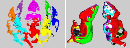
Fig. 1.7 Example of model reconstruction. Partial 3D views of the object of interest are acquired (left). After registration all the 3D views are transformed to the common reference system and merged (right). Figure generated by Alessandro Negrente, reproduced from [17]
high quality correspondences can be established. Over the last two decades, many variants of ICP have been proposed to improve the speed and accuracy of the registration process. An example of the registration required for model construction from partial 3D views is given in Fig. 1.7.
1.5.8Passive 3D Imaging: The Fundamental Matrix and Camera Self-calibration
In 1992 Luong, Faugeras, and Maybank extended the Essential Matrix to uncalibrated cameras through the Fundamental Matrix. While for the Essential Matrix estimation, the camera intrinsic parameters had to be known in advance, now arbitrary cameras could be used and calibrated from the image data alone. The papers by Faugeras:What can be seen in three dimensions with an uncalibrated stereo rig? [13] and by Faugeras, Luong and Maybank: Camera self-calibration: Theory and experiments [14] started a new research area within computer vision that today allows us to reconstruct large 3D environments from arbitrary image collections; for example, those taken by tourists and uploaded to the web. There are even web services available that enable us to simply upload our pictures of a scene and obtain 3D representations from them.
The basic algorithm for estimating the Fundamental Matrix from 8 correspondences was rather sensitive to correspondence errors and researchers were sceptical about its usability in noisy imaging conditions. This problem was tackled in 1995 by Richard Hartley in his famous work entitled In Defense of the 8-Point Algorithm [22] [23]. Hartley showed that image normalization is vital for practical Fundamental Matrix estimation.

20 |
R. Koch et al. |
1.5.9 3D Local Shape Descriptors: Spin Images
The ICP algorithm fails if it converges to a local minimum that is not the global minimum of the least-squares registration error. A common approach to prevent this is to determine a sparse set of three or more strong local descriptor (feature) matches across the pair of 3D shapes, which allows coarse 3D registration to within the convergence basin of ICP. Probably the most well-known 3D local shape descriptor is the spin image [26], presented by Johnson and Hebert in 1997. Here the local normal of a 3D point is used to encode neighbouring points by measuring their height in the direction of the normal and their radius in the tangential plane described by the normal. Thus a spin image encodes the relative positions of neighboring points in a cylindrical-polar coordinate system. The neighbor’s angles in the tangential plane are discarded in order to give pose-invariance to the descriptor and the heights and radius values of the neighbors are built into a two-dimensional histogram, which forms the spin image descriptor. A large number of experiments in the literature have shown that the spin images are powerful for several tasks that include the registration of overlapping shapes, 3D object recognition and 3D shape retrieval (shape search).
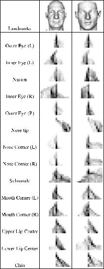
Figure 1.8 shows some examples of spin images computed on 3D captures of human faces [11]. In this case, the spin images are taken over a limited local range, as the 3D face surfaces are partial scans taken from a single viewpoint (there is no scanned surface for the back of the head). In the figure, the spin images for a given landmark appear quite similar across two different faces. For complete 3D scans, it is possible for spin images to encode the full extent of the object.
1.5.10 Passive 3D Imaging: Flexible Camera Calibration
Camera calibration is the process whereby intrinsic camera parameters are established, such as the focal length of the lens and the size and aspect ratio of the image sensor pixels. The position and orientation of the camera relative to the scene is also established and the parameters describing this are referred to as extrinsic parameters. Many current approaches to camera calibration are based on the easy-to-use, yet accurate approach presented by Zhang in 2000,22 where calibration can be achieved from n-views of a calibration grid of known grid dimensions [57]. This calibration grid is a planar ‘chessboard’ pattern of alternate black and white squares which can be freely moved as the calibration images are captured, the motion between the captures is not required, hence the system is easy
22Zhang’s seminal work is pre-dated by a large body of pioneering work on calibration, such as D.C. Brown’s work in the context of photogrammetry, which dates back to the 1950s and many other works in computer vision, such as the seminal two-stage method of Tsai [53].
1 Introduction |
21 |
Fig. 1.8 Example spin images computed for 14 landmarks on two different faces from the FRGC dataset. Here a bin size of 5 mm is used. The size of the spin image is 18 × 9 pixels. The middle top part of the spin image is the 3D surface point whose local shape we are encoding; the left part of the spin image corresponds to points above this 3D point in the direction of the normal; the right part corresponds to points below, using this same direction. The vertical direction in the spin image corresponds to the radius in the tangential plane. Figure adapted from [11], courtesy of Clement Creusot
to use. Although the minimum number of images captured is 2, around 20 are commonly used for improved accuracy. The estimation is in two-stages: firstly, a closed-form linear solution for the camera’s parameters is used, followed by a non-linear refinement based on the maximum-likelihood criterion. In the first stage, lens distortion is assumed to be zero, whereas the second stage provides a mechanism for radial distortion parameters to be estimated, if required. Figure 1.9 illustrates a typical set of calibration plane positions to calibrate a camera and a standard corner detector is used to find each junction of four squares on each chess-