Материал: Russian Journal of Building Construction and Architecture

A heat pump turns on in cycles with alterations of a supply (removal) of heat with stops. For the second stage, i.e. the cooling stage, the initial conditions are a complex temperature field formed during stationery operation of the heat pump over the first calculation period 0 < < 1:

where τ1 is the operation time of the heat pump setup of the second stage, sec.

For the third stage, i.e. when the heat pump turns on following a stop, the initial conditions for calculations will be a complex temperature field obtained following the cooling of the layer

1< < 2:

where τ2 is the operation time of the heat pump setup of the third stage, sec.

The boundary conditions at the face of the well are accepted depending on the technological modes of the first, second, and third order:

–– first order, where there is no influence of the wells and constant temperature

t ( , τ) = tbackground;

–– second order, on the surface of the casing pipe of the well; for the operating heat pump:

t(rc , ) q ;r

and for the non-operating heat pump:

t(rc , ) 0;

r

–– for the second order, on the lower generating line of the calculation cylinder, the earth’s warmth, the heat flow is considered constant:

t(r, ) q ;r

–– the third order, on the Earth’s surface, due to a significantly larger thermal conductivity coefficient on the surface in relation to the heat transfer coefficient of a soil from the surface to the heat exchange part of the well can be changed by the first order: t (r, ) = tclimate.

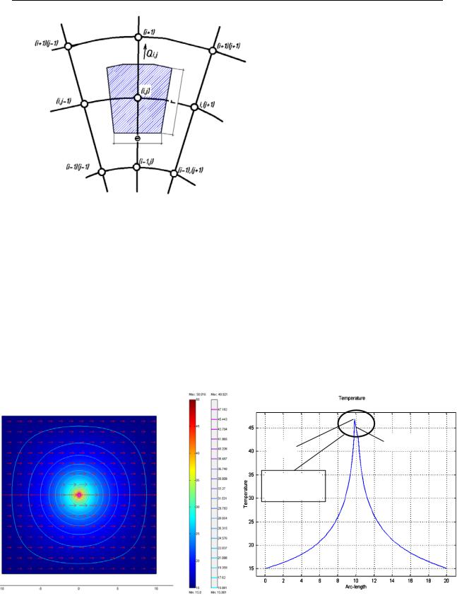
The solution for modeling a temperature field is obtained by means of the method of finite differences using an implicit difference scheme (Fig. 2) [8].

The equation (2) in the discrete form is as follows:

where i, j are the indices (numbers) of the corresponding nod point along the axis Х and У.

61

Russian Journal of Building Construction and Architecture

Fig. 2. A grid and a control volume in polar coordinates r, ϴ

2. Calculation prediction of the distribution of temperature fields considering a filtration flow of groundwater

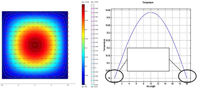
Determining the effect of a filtration flow of groundwater is reduced to solving the problem of flowing of a circular cylinder. In Fig. 3—6 there are the results of the influence of groundwater during the operation of the well for 5 years for a heat load on the well of 200 Watt seasonally. The prediction results are performed using a numerical model implemented using the applied software MathLab.

TPeak TAxis

Displacement

of the field

Fig. 3. Results of the operation of a heat pump setup over 6 months:

а) a temperature field of the soil; b) a temperature graph in direction to a filtration flow;

Тaxis is the temperature along the well axis; Тpeak is the peak temperature of the soil in operation over 6 months

62

As seen from Fig. 3, a heat flow is distributed radially from the well. In Fig. 3b the temperature graph is displaced in relation to the main axis of the well (the area is 10 meters and it is accepted to be the centre of the well) along the axis Х, the deviation is close to 0.3 m.

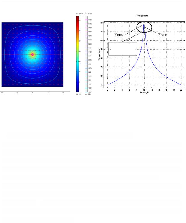
Fig. 4 shows the results of the experiment of the first year of the operation when the heat pump is not in operation (the downtime period).

As seen from Fig. 4а, the distribution of a heat flow is radial similarly to Fig. 3. As during the downtime period the heat pump is not in operation, the temperature field around the well yields to the background temperature of the soil.

The boundaries of the temperature graph (Fig. 4b) from both sides of the axis approach the contour of the influence of the external boundary if the task is accepted to be along the radius and is 10 m. Thus when the heat pump setup is not in operation, there is no displacement along the main axis under the influence of a filtration flow.

Approaching the influence boundaries

Fig. 4. Results of the first year of the operation of the well during the downtime period of the heat pump setup: а) a temperature field;

b) a graph of a change in the temperature in direction to a filtration flow

As the operation time increases, there is no displacement along the axis Х. Stabilization of the temperature of the soil in operation takes place as early as during the second year of the seasonal operation of the heat pump setup.

63

Russian Journal of Building Construction and Architecture

Displacement

of the field

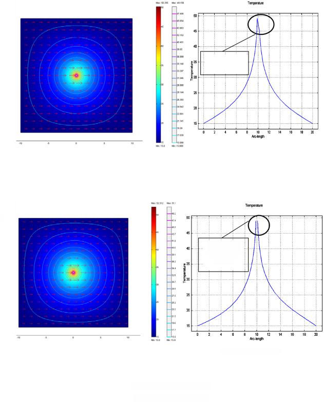
Fig. 5. Results of the operation of the heat pump setup over 3.5 years:

а) a temperature field of the soil; b) a temperature graph in direction to a filtration flow Тpeak is the peak temperature of the soil in operation over 6 months

3. Summarizing the obtained results for more complex filtration

The obtained results for different operation modes of the heat pump setup are processed in order to come up with a method of dependencies for engineering and technical and economic calculations [8]. Fig. 6 presents the temperature fields and graphs for different rates of groundwater. In order to allow the results to be further employed in experimental and theoretical studies of a wide range of engineering objects, the similarity theory was used.

Fig. 7 presents the results of the effect of the filtration rate on heat exchange. To make it easier for the obtained data to be processed, the following dimensionless values are introduced as part of the study: С is the criterion of the multiplicity coefficient of water exchange, θ is a dimensionless temperature, Q is a dimensionless heat flow, P is a correction for a filtration flow, kP is a regeneration coefficient.

As seen from the graph, there are two modes. The first mode is when the filtration rate is slow and has no effect on a temperature field, the second one is when as the filtration rate is on the rise, the temperature pressure drops.

Based on the processing of the obtained results, the correction modes were identified. If 0 < С < 78, P = 1, a filtration flow has no effect, if C > 78, a filtration flow has an effect on the temperature of the soil.

64

I

Displacement

of the field

II

Break along the length of the well

Fig. 6 (beginning). A field and a temperature for different rates of groundwater:

I — υ = 0,000000001 m/seс;

II — υ = 0,00000009 m/sec

65