Материал: Крючков Фундаменталс оф Нуцлеар Материалс Пхысицал Протецтион 2011

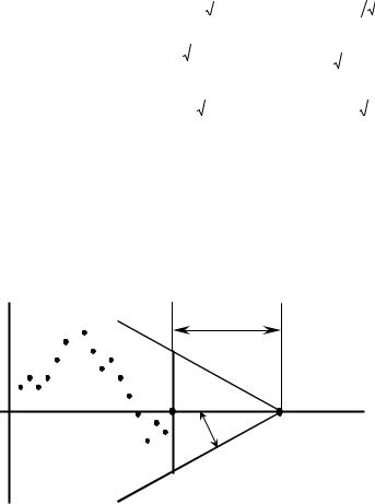
Table 4.9

Control limits for various statistics

Cumulative sum chart (diagram)

Shewhart charts largely help control retrospectively single and rather great anomalies in a process. A process may however involve minor but permanent biases desired to be controlled on line rather than retrospectively. Cumulative sum diagrams (CUSUM) help detect such deviations rapidly (Fig. 4.7).

A'

d

A

θ О

B

B'

Fig. 4.7. Example of a CUSUM chart

For a CUSUM diagram, the subgroup number is plotted on the abscissa axis and the cumulative sum value for the deviations from the mean value (or a standard quantity) is plotted on the ordinate axis:

216

m

T m = ∑(Y i − μ 0) . (4.76)

i =1

If the process is in control and there are no systematic biases and/or thefts, Tm is expected to vary around zero. If any systematic factors arise in the process (in this case the points in the Shewhart chart are on the one side of the center line), the CUSUM curve will have an upward or a downward trend.

A special note should be made that scale is critically important to the CUSUM diagram plotting. To have points well discernible and make it easier to plot the so-called V-mask, the recommendation is that the distance between points on the abscissa axis should be in a range of σY ÷ 2,5 σY. Scale observation is very important since this is what the mask angle depends on. Selecting an acceptable scale helps get the mask angle θ in a range of 30–60 °, which, in turn, ensures the best outcome and helps escape errors which are inevitable if the selected angle is too small or too great.

The process control procedure is as follows. The mask (the procedure to plot the V-mask will be discussed hereinafter) is superimposed on the diagram so that the point P falls on the farthest diagram point and the line OP is parallel to the abscissa axis. If none of the diagram point falls beyond the limits of the angle A'OB', the process is assumed to be in control.

To be plotted, the V-mask requires two elements: angle, θ, and distance,

d:

where σ is the sample-mean variance; D is the bias quantity (either in one direction or in the other) to be found with the specified probability; δ is the

scaling factor that determines the control chart geometry and the mask size;

217

where E(α) is the coefficient which is the function α (the probability of a first-order error). The values of this coefficient are given in Table 4.10.

Table 4.10

Factor values E(α) depending on the probability of a first-order error

So, plotting a CUSUM diagram and estimating the process stability involves the following steps:

1)selection of a suitable axis scale, plotting of experimental points on the CUSUM diagram;

2)selection of α and δ, calculation of σ, determination of the V–mask parameters (θ and d), mask plotting;

3)the mask is placed on the control chart as described hereinabove and all points are checked left of the mask’s point P, the upper mask ray being the lower control limit and the lower mask ray being the upper control limit.

Therefore, control charts are a powerful tool of finding out and analyzing a certain (other than random!) cause of a deviation, a bias or a process instability, say, an organized NM theft.

There are currently rather many computer programs enabling automated data analysis based on control charts.

References

1.Гераскин Н.И., Петрова Е.В. Теория вероятностей и прикладная математическая статистика в задачах физической защиты ядерно– опасных объектов, учета и контроля ядерных материалов. М.: МИФИ, 2001.

2.Колмогоров А.Н. Основные понятия теории вероятностей. М.:

Наука, 1974.

3.Вентцель Е.С. Теория вероятностей. М.: Высшая школа, 1998.

4.Основные правила по учету и контролю ядерных материалов (ОПУК). НП–030–05. Утверждены Постановлением Федеральной службы по экологическому, технологическому и атомному надзору N 19 от 26 декабря 2005 года. М., 2005.

218

5.Кассандрова О.Н., Лебедев В.В. Обработка результатов наблюдений. М.: Наука, 1970.

6.Deming W.E. Some Theory of Sampling. Dover Publications Inc. New York, 1998.

7.Reilly D., Ensslin N., Smith H., Jr., Kreiner S. Passive Non– Destructive Assay of Nuclear Materials. NUREG/CR–55 50, LA–UR–732.

8.Худсон Д. Статистика для физиков. М.: Мир, 1970.

9.Ильенкова С.Д., Ильенкова Н.Д. и др. Управление качеством. М.:

ЮНИТИ, 1998.

219

CHAPTER 5

MEASUREMENTS OF NUCLEAR MATERIAL FOR ACCOUNTING AND CONTROL THEREOF

This Chapter reviews and looks into the techniques and equipment used to account for and control nuclear material (NM). The nuclear material subject to control is listed, and the properties thereof and the conditions of test measurements are discussed.

The most common destructive and nondestructive test techniques, as well as passive and active analyses are described. Most of the test techniques are based on recording of gamma and neutron radiation. Data on detectors and equipment employed, as well as on calibration procedures and standards is provided. Sources of measurement errors and measures to reduce these are discussed. In conclusion, examples of combined NM measurement methods used in production are given.

5.1. Basic concepts of NM measurements

Prior to the 1990s, onsite NM measurements were conducted in Russia largely for control of processes. Nondestructive assays (except weighing) had minor roles.

In the 1990s, comprehensive measures began to be undertaken in Russia to have nondestructive assay (NDA) techniques more rapidly introduced into the Russian NM accounting and control system, including by way of providing enterprises and organizations with up-to-date devices, developing and qualifying state standard samples for NDA, creating respective regulatory documentation and training personnel through a variety of educational forms. Major emphasis in this has been also placed on international cooperation.

Russian requirements with respect to state accounting and control of nuclear material in production, utilization, processing, storage and transportation are set forth in the General Rules for Accounting and Control of Nuclear Materials, NP-030-05 (OPUK-2005).

As weapon grade nuclear material, uranium and plutonium prevail. Weapon Grade Uranium (WGU) contains 93% or more of 235U.

Weapon Grade Plutonium (WGPu) is a pure plutonium metal that contains not more than 7% of the 240Pu isotope.

Reactor Grade Plutonium (RGPu) accumulates in fuel of power reactors and contains 19% of 240Pu isotope or more. The approximate isotopic

220