Материал: Крючков Фундаменталс оф Нуцлеар Материалс Пхысицал Протецтион 2011

Kurchatov’s may entail estimated at a level of 60 to 70 man-years. The initial physical inventory to be taken at Kurchatov’s is expected to last for several years.

It needs to be said that the labor consumption in physical inventory takings can be decisively curtailed to a great extent by means of access controls (containment and surveillance), provided these are employed as extensively as they can be. Estimates show that access controls, if applied to the nuclear material of the Kurchatov’s facilities, are expected to make the volume of routine physical inventory takings (not of initial ones) several times smaller. Thus, a five times reduction in this value means that all this work can be done by a team of 6 or 7 persons in approximately 2 years.

Manning problem

Manning problems are faced by many operators within the Russian nuclear fuel cycle. It needs to be acknowledged so that lack of sufficient personnel to have NM physical inventories taken in Russia in near future is rather a concern. Later on, however, things with this can be somewhat settled thanks to a reduction in the overall labor expenditures after the initial PITs are completed given access controls are employed.

Early physical inventories takings led to the understanding that even expert staff who were or are involved in building the existing economical and safe nuclear facilities have proved to be unable to elaborate and use the physical inventory taking procedures without being given a prior special training. The explanation is that a physical inventory taking is actually a sort of a global physical experiment, so the absolute must for Russia now is a well-established framework for training and retraining personnel to operate the NM accounting, control and physical protection system.

Nuclear material balances

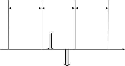
We shall assume that the site under consideration has periodic NM physical inventories taken thereat (Fig. 6.1). The period of time Т between the two successive physical inventory takings is called the material balance period.

Let we know the physical inventory PI of the material in the given material balance area as of the time t0 of the previous physical inventory taking and that IN of material was received in the given MBA over the material balance period Т. This is exactly the quantity of the material the receipt whereof has been booked in records.

296

Similarly, DE is the quantity of the material shipped from the given balance material area over the period (t0, t1) between the physical inventory takings.

MPB

Fig. 6.1. NM balance closing cycle in an MBA

The book inventory of the nuclear material is the quantity of the nuclear material to be present in the MBA as shown in the documents as of a particular date. The final book inventory BI of the material in the given material balance area as of the current physical inventory taking time is evidently:

The physical inventory EI of the nuclear material is the quantity of the material as determined in the course of the current physical inventory taking by measurements and computations.

The difference between the book inventory BI of the material as of the current PIT time and the physical inventory EI is called the inventory difference (ID). The objective of the nuclear material balance closing is to find the ID.

The following equation gives a formal determination of the inventory difference ID:

297

The equation (6.2) is the basic balance relation. This equation should be solved on a periodic basis for each material balance area. It is solved for separate types of the NM held within the MBA concerned. Let us remind that the NM type is the nuclear material the isotopic composition whereof is in the given interval limits (e.g., uranium, uranium-235, plutonium, etc.).

Statistical interpretation of the nuclear material balance

The inventory difference cannot be avoided because of unavoidable measurement system errors. It may both positive and negative.

In a general case, the values I, EI, IN and DE in equation (6.2) are found experimentally and contain systematic and random measurement errors. The measured values I, EI, IN and DE are not negative random values having certain probability density distributions. The total value ID is also a random quantity, either negative or equal to zero, having a certain probability density distribution as generated by the superposition of the probability density distributions of the quantities I, EI, IN and DE.

Equation (6.2) has three important sequences.

1)The quantity ID is the superposition of multiple random quantities and so, according to the central limit theorem, its distribution is close to normal (Gaussian distribution). In this case, the bounds of the 95% and 99% confidence intervals are determined easily depending on σID.

2)The inventory difference (ID) is linear relative to the components thereof. This circumstance will be further used to plot calculation models

for σID.

3) If the terms of equation (6.2) are independent variables, then the statistical straggling of the ID is described by the quantity

To determine the quantity of the ID’s mean-square error, the “measurement error carry” technique shall be prefer ably employed. This consists in that the inventory difference errors are computed from the measurement errors for the quantities in the NM balance equation. Also taken into account are random and systematic components of errors and potential correlations of the NM characteristic measurement errors.

It should be noted that where a great deal of measurements is involved in the components of equation (6.3), Var (ID) may amount to an intolerably great quantity. The approach with the division of measurements into accounting and verifying ones, as taken in the measured material balance

298

system, enables the problem of great ID variances to be removed to a certain extent. To this end, the material balance equation (6.2) is considered by components. The NM available for the MBP under consideration may be classified as follows.

Passive NM is the material that has not been changed in any way (and has been under access controls) over the MBP preceding the given PIT. It is subject to verifying measurements during the PIT.

Active NM is the NM that has had its state changed and have undergone or is subject to accounting measurements (processing, change of accounting data, etc.).

Examples of passive and active NM determination

1)A storage facility for unirradiated NM. All material is under TIDs. Over the MBP, material was received at and shipped from the storage facility. How shall the material left as of the time of the next PIT be classified?

2)A process department for uranium dioxide production out of uranium hexafluoride is considered. There was no nuclear material in the MBA as of the previous PIT time. Over the MBP, cylinders with UF6 were received from which UO2 was produced, containerized and shipped to another department. As of the time of the current PIT, the MBA had cylinders with UF6 remainder and containerized UO2 left therein. Shall all NM be classified as active?

Anomalies in accounting of NM are revealed in the course of physical inventory takings and material balance closing. For the above NM classes, the following criteria for detection of anomalies in accounting and control of NM are considered.

Passive NM balance closing

The anomaly for passive NM is the discrepancy in accounting and verifying data to above the permissible limits. In this case, a new accounting measurement of NM is performed. Where the accounting data is verified, this NM changes neither ID nor the ID uncertainty. Therefore, with anomalies absent in the verifying measurements:

ID = IDACT; Var(ID) = Var(IDACT).

Active nuclear material balance closing and inventory difference determination

For active NM, in a general case, the conclusion on the balance arrived at, based on the coincidence of the IL and the PIL for each item, cannot be

299

made due to active NM being subject to change during the MBP. So in the event of active NM, an integral criterion for the conformity of the accounted for and physical NM remainder in the MBA as of the current PIT time is considered. The inventory difference quantity acts as this criterion.

The active NM balance closing suggests that the IL and PIL conformity should be established both in the number of products and in attributes. Apart from this, the inventory difference and its limiting values should be determined for active nuclear material. A correct evaluation of the inventory quantity requires waste, loss, discard and NM deposition in process equipment to be taken into account.

For active NM, the anomaly is the IL/PIL discrepancies in the number of items or attributes thereof. The integral criterion of the anomaly detection is the modulus in excess of the inventory difference or its threefold mean-square error, or the values of any of the following quantities, the confidence probability being 0.95:

∙2% of the total book inventory of the given nuclear material and all quantity increases thereof over the MBP for commercial nuclear facilities;

∙3% of the same quantity for nuclear research facilities;

∙3 kg of plutonium or uranium–233 in the MBAs that c ontain category 1 and 2 nuclear material;

∙8 kg of uranium–235 in the MBAs that contain catego ry 1, 2 and 3 nuclear material;

∙70 kg of uranium–235 for uranium enriched to below 20%.

Limits of allowable ID deviations based on accounting of NM measurement errors

Let us assume that the ID is characterized by normal distribution. We shall designate

Two intervals are considered to analyze the allowable ID values. The

interval (–2 σ , +2σ ) is a 95% confidence interval. The interval (–3 σ ,

ID ID ID

+3σ ) is a 99% confidence interval:

ID

a)95% confidence interval. The probability of this interval being exceeded is small (0.05). It defines the bounds (warning limit) of the statistically insignificant ID straggling range.

b)99% confidence interval. The bounds of this interval define the permissible ID values. The frequency of false signals for such interval is

300