Материал: Маслов ИНТРОДУЦТИОН ТО ПХЫСИЦС ОФ СЕЦОНД-ОРДЕР МАГНЕТИЦ 2015
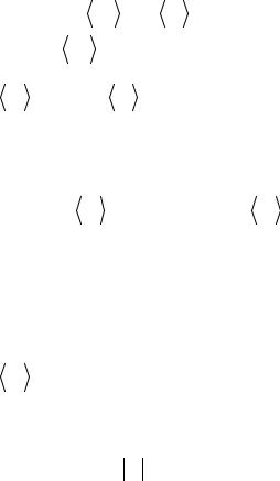
can denote |
|
as |
|
, the same for all j . Then the term |
σjz |
σz |
∑ |
/ |
|
|
|
|
|
in |
the |
|
Hamiltonian |
|
takes |
the |
form |
||
|
Jij σiz |
σjz |
|
|
|
|||||||||||
i, j |
|
|
|
|
|
|
|
|
|
|
|
|
|
|
|
|
|
|
∑ |
/ |
|
|
|
N |
N |
|
Recall that Jij |
= J (Ri − Rj )= J (Rl ), |
|||||
σz |
|
Jij σiz |
= σz ∑∑Jij σiz . |
|||||||||||||
|
|
i, j |
|
|
|
|
i=1 |
j≠i |
|
|
|
|
|
|
|
|
where Rl |
= Ri |
− Rj |
is the vector drawn from j-th magnetic moment to i- |
|||||||||||||
th, and convert the sum ∑ to ∑ in the interaction term |
|
|||||||||||||||
|
|
|
|
|
|
|
|
j≠i |
l ≠0 |
|
|
|
|
|
|
|
|
|
|
|
|
|
N N |
|
|
|
|
N |
/ |
|
|
(11.7) |
|
|
|
|
|
|
σz ∑∑J |
(Ri − Rj )σiz = σz |
∑∑ |
|
J (Rl |
)σiz , |
||||||
|
|
|
|
|
|
i=1 |
j≠i |
|
|
|
|
i=1 l |
|
|
|
|
where ∑/ is the sum for all vectors Rl |
that drawn from arbitrary atom |
|||||||||||||||
|
|
|
l |
|
|
|
|
|
|
|
|
|
|
|
|
|
(magnetic moment) to all other atoms (magnetic moments), the prime implies that Rl ≠ 0. This sum is the same for every atom, since we con-
sider that all atoms (magnetic moments) located periodically, i.e., they form the crystal. Thus, the interaction term takes the following form
|
∑ |
/ |
|
N |
|
where ∑ |
/ |
J (Rl ) is the certain characteristic en- |
σz |
|
J (Rl )∑σiz , |
|
|||||
|
l |
|
|
i=1 |
|
l |
|
|
ergy (sum of the energies of exchange interactions of randomly selected atom with all other atoms). Taking into account that J (Rl ) falls off ex-
ponentially as the Rl increases, denote the J (Rl )= J for the nearest neighbors and considering that J (Rl )= 0 for other atoms, we obtain ∑/ J (Rl )≈ zJ, where z is the number of nearest neighbors of each
l |
|
atom (magnetic moment). Since J = (0.001÷0.1) eV, zJ |
may take the |
sufficiently large values zJ = (0.1÷1) eV. Denote this energy as |
|
∑/ J (Rl )= kBθ, |
(11.8) |
l |
|
26

where θ is the some characteristic temperature (next, we shall omit the Boltzmann constant).
Thus, taking into account the notation introduced, we can write down the Hamiltonian of the Ising model in the following form
|
|
N |
N |
= E0′ |
|
N |
(11.9) |
H = E0′ − |
σz |
θ∑σiz − h∑σiz |
−(θ σz |
+ h)∑σiz . |
|||
|
|
i=1 |
i=1 |
|
|
i=1 |
|
Denote the “effective field” heff |
|
|
. So, the Hamiltonian of the |
||||
= h + θ σz |
|||||||
Ising model can be described as |
N |
|
|
|
|||
|
|
|
E0′ − heff |
|
|
(11.10) |
|
|
|
H = |
∑σiz . |
|
|||
i=1
The main differences between this Hamiltonian and the Hamiltonian
|
N |
are the appearance |
of noniteracting magnetic moments H0 |
= −h∑σiz |
i=1
of the constant E0′ (note that E0′ does not affect on the  σz
σz  calculation)
and the field h substituted by the “effective field” heff = h + θ σz
σz  .
.
Finally, in the mean-field approximation system of interacting magnetic moments can be approximately described as the system of nonin-
teracting magnetic moments placed into the “effective field” heff ≠ h.
12. Curie-Weiss equation and Curie-Weiss law
We now apply the mean-field approximation to the system of magnetic moments with Jij ≥ 0 (i, j) . In particular, we assume Jij = J
for the nearest neighbors and Jij = 0 for other atomic pairs. Magnetization of such system (projection on the z-axis) equals to
|
|
|
|
N |
|
|
|
|
|
|
|
|
|
M = |
µz |
= |
NµB x |
, |
(12.1) |
||
|
|
|
|
V |
V |
|||||
|
|
|
|
|
|
|||||
where |
µB . The parameter x does not depend on i , |
|||||||||
x = σz |
= µz |
|||||||||
−1≤ x ≤1, and x = 0 in the case of  µz
µz  = 0. Let us find x = x(T, H ).
27
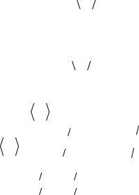
Recall that the Hamiltonian of the Ising model in the mean-field approximation is
|
N |
(12.2) |
H |
= E0′ − heff ∑σiz . |
i=1
N
Constant E0′ does not affect on the  σz
σz  calculation, term −heff ∑σiz is
i=1
the operators sum of the interaction between each magnetic moment and “effective field”. In other words, in our approximation magnetic moments do not depend on each other, but they located in the “effective
field” heff . Therefore, the value  σz
σz  for arbitrary magnetic moment can be obtained in terms of single magnetic moment located in the field
heff . Hamiltonian for the single moment located in the field
|
|
|
|
|
can be obtained as follows |
|||||||||||||
H |
= −heff σz . Therefore |
σz |
||||||||||||||||
|
|
|
|
|
−H T |
|
|
|
|
|
|
) |
|
|||||
|
|
|
Tr (σze |
|
|
|
) |
|
|
Tr (σze |
|
|
||||||
|
|
|
|
ˆ |
|
|
heff σz T |
|
||||||||||
|
|
|
|
|
|
|
|
|
|
|
|
|
|
|
||||
|
σz = |
|
|
|
|
|
|
|
= |
|
|
|
|
|
|
= |
||
|
|
|
Tr |
(e−H T ) |
|
|
|
Tr (eheff σz |
T ) |
|
|
|||||||
|
|
eheff |
T |
−e−heff |
T |
|
heff |
|
|
|
||||||||
|
= |
|
|
|
|
|
|
|
= tanh |
|
|
|
. |
|
|
|||
|
|
h |
T |
+ e |
−h |
T |
|
T |
|
|
||||||||
|
|
e eff |
|
|
eff |
|
|
|
|
|
|
|
||||||
heff is
(12.3)
Recall that the heff = h + θ σz
σz  ≡ h + θx . Therefore the Eq. (12.3) takes the form
h + θx |
(12.4) |
||
x = tanh |
T |
|
|
|
|
|
|
Such dependence of x is referred to as Curie-Weiss equation.
Let us find the magnetization and magnetic susceptibility at high
temperatures T h + xθ . At high temperatures |
h + θx |
→ |
h + θx |
, |
||||
tanh |
T |
|
T |
|||||
|
|
|
|
|
|
|
||
therefore |
x ≈ h + θx |
. Finally, we obtain |
|
|
|
|
|
|
|
T |
|
|
|
|
|
|
|
28
x = |
|
|
h |
|
|
|
= |
|
µB H |
, |
|
|
(12.5) |
||||||||
|
T −θ |
|
T −θ |
|
|||||||||||||||||
|
|
|
|
|
|
|
|
|
|
|
|
||||||||||
M = |
Nµ |
B |
x |
= |
|
Nµ2 |
H |
, |
(12.6) |
||||||||||||
|
|
|
|
|
|
|
|
|
|
B |
|
|
|
|
|||||||
|
|
V |
|
|
|
|
V |
|
T |
−θ |
|||||||||||
|
|
|
|
|
|
|
|
|
|
|
|
|
|
||||||||
χ = |
M |
|
= |
|
NµB2 |
1 |
|
. |
|
(12.7) |
|||||||||||
H |
|
|
|
V |
|
|
|
T −θ |
|
||||||||||||
The latter temperature dependence of χ is referred to as Curie-Weiss law. Note that if the exchange interaction is absent ( Jij = 0 ), then
θ = 0 , so, we obtain the Curie law. The value θ is called the Curie temperature.
13. Ferromagnetic transition in the Ising model. Curie temperature. Order parameter
In the previous paragraph we have shown that at high temperatures
magnetic susceptibility χ = |
NµB2 |
1 |
. One can see that the value of χ |
||||||||||||
|
V |
|
|
T −θ |
|||||||||||
diverges at T → ∞. |
This is due to a violation of the conditions of ap- |
||||||||||||||
plicability |
of our solution. Indeed, we obtained that x = |
µB H |
, i.e., |
||||||||||||
T −θ |
|||||||||||||||
|
T → θ. |
|
|
|
|
|
|
|
|
|
|
|
|||
x → ∞ at |
Therefore |
the |
condition |
T h + xθ |
is |
not |
valid. |
||||||||
However, |
one can |
see that |
some |
“critical” |
temperature |
θ |
exists at |
||||||||
which something happens. Maybe it is a transition to ferromagnetic state? Let us study the Curie-Weiss equation in more detail.
Consider the h = 0 in the Curie-Weiss equation, thus the latter takes the following form
|
θ |
(13.1) |
|
x = tanh x |
|
. |
|
|
|||
|
T |
|
|
This equation can not be solved analytically. We shall try to solve it graphically. From the Fig. 13.1 and 13.2 one can see that at T > θ the Curie-Weiss equation has only one solution ( x = 0 ), but at T < θ it has three solutions ( x = 0; x ≠ 0 ).
29
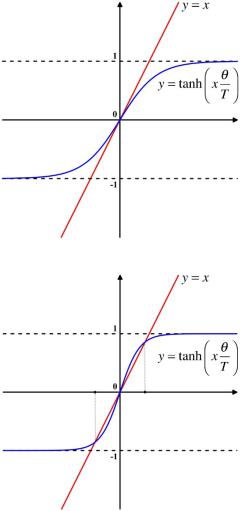
Fig. 13.1. Graphic solution of the Curie-Weiss equation at T > θ
Fig. 13.2. Graphic solution of the Curie-Weiss equation at T < θ
Thus, the main conclusion is that at T = θ = ∑/ J (Rl )≈ (10 ÷1000) K
l
the phase transition into ferromagnetic state occurs, i.e., at T > θ and H = 0 we obtain M = 0 (paramagnetic phase), and at T < θ and H = 0
30