Материал: part17

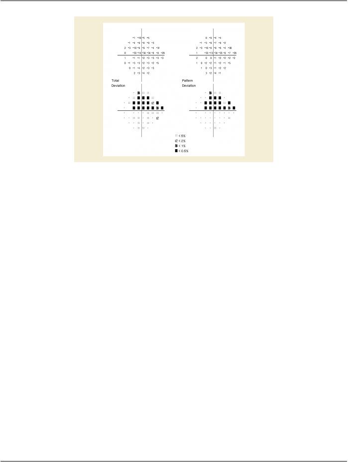
Figure DDD.2-5. Examples of Age Corrected Deviation from Normative Values (upper left) and Mean​ Defect Corrected Deviation from Normative Data (upper right)​

For all normalized visual field sensitivity data, it is useful to know how a particular value compares to a group of normal patients.​ Vendorsofautomatedvisualfieldmachinesthereforegotogreatlengthstocollectdataonsuch"normal"subjectstoallowsubsequent​ analysis. Furthermore, the various sets of values mentioned above can be summarized further using calculations like a mean and​ standard deviation. These values give some idea about the average amount of field loss (mean) and the focality of that loss (standard​ deviation).​

A final step in the clinical assessment of a visual field test is to review any disease-specific tests that are performed on the data. One​ such test is the Glaucoma Hemifield Test, which has been designed to identify field loss consistent with glaucoma. These tests are​ frequently vendor-specific.​

DDD.2.2 Neurological Disease​

In addition to primary diseases of the optic nerve, like glaucoma, visual fields are useful for assessing damage to the visual pathway​ occurring between the optic chiasm and occipital cortex. There is the same need for demographic information, for assessment of re-​ liability, and for the various raw and normalized sensitivity values. At this time, there are no well-established automated tests for the​ presence of neurological defects.​

- Standard -​

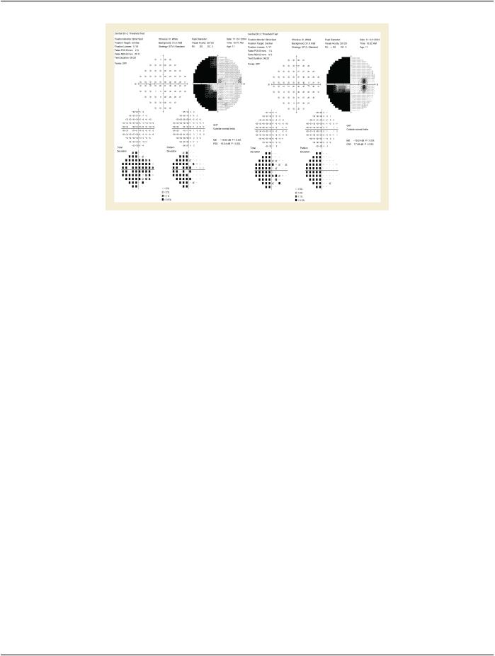
FigureDDD.2-6.ExampleofVisualFieldLossDuetoDamagetotheOccipitalCortexBecauseofaStroke​

DDD.2.3 Diffuse and Local Defect​

DDD.2.3.1 Diffuse Defect​

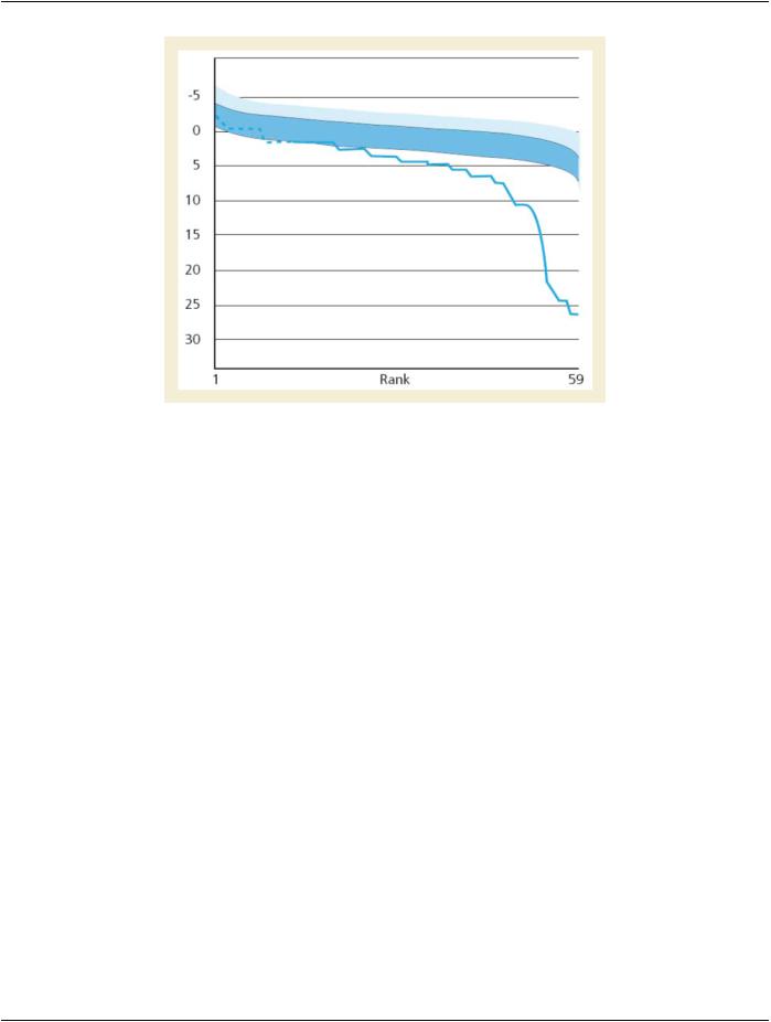
The Diffuse Defect is an estimate of the portion of a patient's visual field loss that is diffuse, or spread evenly across all portions of​ the visual field, in dB. In this graphical display, deviation from the average normal value for each test point is ranked on the x axis​ from 1 to 59, with 59 being the test point that has the greatest deviation from normal. Deviations from normal at each test point are​ represented on the y axis, in dB. The patient's actual test point deviations are represented by the thin blue line. Age corrected normal​ values are represented by the light blue band. The patient's deviation from normal at the test point ranked 25% among his or her own​ deviations is then estimated to be his or her diffuse visual field loss, represented by the dark blue band. This provides a graphical​ estimate of the remaining visual field loss for this patient, which is then presumed to consist of local visual field defects, which are​ more significant in management of glaucoma than diffuse defects.​

- Standard -​

Figure DDD.2-7. Example of Diffuse Defect​

DDD.2.4.2 Local Defect​

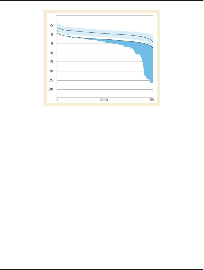
The Local Defect is an estimate of the portion of a patient's visual field loss that is local, or not spread evenly across all portions of​ the visual field. The x and y axis in this graphical display have the same meaning as in the diffuse defect. In this graphical display the​ top line/blue band represent age corrected normal values. This line is shifted downward by the amount estimated to be due to diffuse​ visual field loss for this patient, according to the calculation in Figure DDD.2-7 (Diffuse Defect). The difference between the patient's​ test value at each point in the ranking on the horizontal axis and the point on the lower curve at the 50% point is represented by the​ dark blue section of the graph. This accentuates the degree of local visual field defect, which is more significant in management of​ glaucoma than diffuse defects. The Local Defect is an index that highly correlates with square root of the loss variance (sLV) but is​ lesssusceptibletofalsepositives.Inadditiontotheusageinwhite/whiteperimetryitisespeciallyhelpfulasearlyidentifierforabnormal​ results in perimetry methods with higher inter subject variability such as blue/yellow (SWAP) or flicker perimetry. An example of Local​ Defect is shown in Figure DDD.2-8 and is expressed in dark blue in dB and is normalized to be comparable between different test​ patterns.​

- Standard -​

Figure DDD.2-8. Example of Local Defect​

- Standard -​

- Standard -​